Forcing Regression Coefficients in R - Part I
Question:
I’m working on a regression model and I need to force the regression coefficients to be positive. How can I accomplish this in R?
Solution:
For linear model regression model with restricted coefficients you have 3 options: Linear with nls, Bayes with brms and Lasso. Here we will look at Linear Model with nls
The function lm does not provide a way to restrict coefficients. Instead we can use the function nls under the algorithm port. This allow us to provide start for the coefficients, as well as upper and lower boundaries.
In order to define the coefficients create arbitrary coefficient names and define them just like I did below. I picked “a” to be my intercept and “b1”,“b2” and “b3” to be my coefficients for the individual variables
# Load libraries
require(tidyverse) #manipulate data
require(knitr) # See Table

# Use formula nls instead of lm and select algorithm port
fit1 <- nls(formula =  Sepal.Length ~ a + b1*Sepal.Width +  b2*Petal.Length + b3*Petal.Width,
    data = iris,
    start = list(a = 0,b1 = 0.0,b2 = 0, b3 = 0),
    lower = c(a = 0,b1 = 0,b2 = 0, b3 = 0),
    upper = c(a = Inf,b1 = Inf,b2 = Inf, b3 = Inf),
    algorithm = "port")

# We see that the coefficients are equal or greater than 0
c.fit1 <- data.frame(t(coef(fit1)))
colnames(c.fit1) <- c("(Intercept)",colnames(iris)[2:4])
knitr::kable(c.fit1, caption = "Forced Positive Coefficients")| (Intercept) | Sepal.Width | Petal.Length | Petal.Width |
|---|---|---|---|
| 2.24914 | 0.5955247 | 0.47192 | 0 |
That’s all
* For Solution with Bayes
* For Solution with Lasso
Want more detail? Then keep reading…
Business Applications:
Marketing Mix,Price Elasticity
In several situations, like building a marketing mix model, I found myself with variables that have to be included in a model but the coefficient ended up with the opposite sign as wanted. It’s very important in these cases to address if there are any other data issues before forcing a coefficient, since this will not make the model optimal from an OLS (Ordinary Least Squares) perspective.
For example, I had cases in which Marketing Tactics such as TV was providing negative effect in sales. While this could be true, it is uncommon to see TV ads that have negative effect in the market. A good remedy is to provide positive priors and regress using bayes approach. That could help the algorithm find I new local minima. You can find such positive priors from correlations between TV and Sales using past data prior to the model, or manually providing industry averages.
Another case is when calculating Price Elasticity. We might find that, as price increases so does sales volume. And again this could be again true if there’s scarcity of the product, or if higher price makes the product look more attractive to consumers. Again, I found myself in the situation where price elasticity did not make sense from a business perspective.
However, this was because I had relatively low number of data points to make my estimation. When prices are very concentrated in a small range, it is very hard to find the actual slope of the regression. To solve this, I first recommend to ask for more data, and if this is not possible and it’s absolutely necessary to provide an answer then I turn to ‘Shrinkage methods’ like lasso.
Detailed Example
# Libraries
require(tidyverse) #Manipulate data
require(DT)        #Visualize data in tables

# Function to visuzalize regression line on plot
reg <- function(x, y, col) abline(lm(y ~ x), col = col)

# Aestethics for the Pairs Plot
panel.lm =  function(x, y, col = par("col"), bg = NA, pch = par("pch"),
    cex = 1, col.smooth = "red", span = 2/3, iter = 3, ...)  {
    points(x, y, pch = pch, col = col, bg = bg, cex = cex)
    ok <- is.finite(x) & is.finite(y)
    if (any(ok)) reg(x[ok], y[ok], col.smooth)
}

# Other Aesthetics, labels and others
panel.cor <- function(x, y, digits = 2, prefix = "", cex.cor, ...)
{
 usr <- par("usr"); on.exit(par(usr))
 par(usr = c(0, 1, 0, 1))
 r <- abs(cor(x, y))
 txt <- format(c(r, 0.123456789), digits = digits)[1]
 txt <- paste0(prefix, txt)
 text(0.5, 0.5, txt, cex = 1.1, font = 4)
}

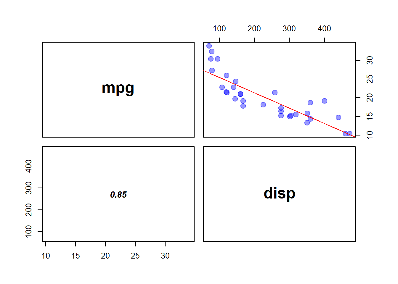
# Variable MPG and Disp show negative correlation
pairs(mtcars[c(1,3)], panel = panel.lm,
    cex = 1.5, pch = 19, col = adjustcolor(4, .4), cex.labels = 2,
    font.labels = 2, lower.panel = panel.cor)
# However when we regress all variables disp has positive slope
lm(mpg ~ ., data = mtcars) %>%
  broom::tidy() %>%
  select(1,2) %>%
  mutate(estimate = round(estimate,4)) %>%
knitr::kable(caption = "OLS Regression Coefficients for dependent variable MPG")| term | estimate |
|---|---|
| (Intercept) | 12.3034 |
| cyl | -0.1114 |
| disp | 0.0133 |
| hp | -0.0215 |
| drat | 0.7871 |
| wt | -3.7153 |
| qsec | 0.8210 |
| vs | 0.3178 |
| am | 2.5202 |
| gear | 0.6554 |
| carb | -0.1994 |
Now let’s force the coefficients to be positive for disp
# Create formula for all coefficients
b_part <- paste0("b",1:(ncol(mtcars) - 1),"*", colnames(mtcars)[-1],
                 collapse = " + ")
formula <- paste0(colnames(mtcars)[1]," ~ a + ", b_part)

# Create List for the restrictions
ab_list <- c("a",paste0("b",1:(ncol(mtcars) - 1)))
start <- rep(list(0),ncol(mtcars))
names(start) <- ab_list
lower <- rep(list(0),ncol(mtcars))
names(lower) <- ab_list
upper <- rep(list(Inf),ncol(mtcars))
names(upper) <- ab_list

# Run the linear Regression with all the restrictions
nls(formula =  formula,
    data = mtcars,
    start = start,
    lower = lower,
    upper = upper,
    algorithm = "port") -> fit3
  fit3 %>%
  broom::tidy() %>%
  select(1,2) %>%
  mutate(term = c("(Intercept)",colnames(mtcars)[-1]),
         estimate_restricted = estimate) %>%
  select(term,estimate_restricted) -> tidy_fit3

lm(mpg ~ ., data = mtcars) -> fit4
fit4 %>%
  broom::tidy() %>%
  select(1,2) %>%
  mutate(estimate_original = estimate) %>%
  select(term,estimate_original) %>%
  inner_join(tidy_fit3, by = "term") -> tidy_fit3

knitr::kable(tidy_fit3, caption = "Linear Regression Coefficients for dependent variable MPG: OLS vs. Forced Coefficient")| term | estimate_original | estimate_restricted |
|---|---|---|
| (Intercept) | 12.3033742 | 0.0000000 |
| cyl | -0.1114405 | 0.0000000 |
| disp | 0.0133352 | 0.0000000 |
| hp | -0.0214821 | 0.0000000 |
| drat | 0.7871110 | 1.2139178 |
| wt | -3.7153039 | 0.0000000 |
| qsec | 0.8210407 | 0.6317301 |
| vs | 0.3177628 | 4.6582898 |
| am | 2.5202269 | 6.0007956 |
| gear | 0.6554130 | 0.0000000 |
| carb | -0.1994193 | 0.0000000 |
So now the question is how much worse is this new model.
If we compare residuals for each model original OLS regression had 12.1447 whereas the restricted model 17.6378.
So clearly the new model is worse. We must keep in mind that this is an extreme case, since we have forced everything to be positive. We should carefully pick what variables should be restricted and which ones shouldn’t.
It’s up to the analyst to consider whether this model is ‘good enough’ to be used for business purposes. What do I mean by good enough? the applications of a regression model are uncountable, and we must consider what is the objective. For instance, we could be trying to assess if there’s any positive effect of variable x on y when we incorporate all the other variables. In that case, even if the model is worse, we would keep the results of the model.
In this case, we are going to assess if the differences are statistically and also visually looking at the predictions.
To test if both models are statistically different we can run an ANOVA test.
# Because nls does not behave well with Anova I create a lm model with forced coefficients. You can better understand this concept [here]()

# Compare Complex model to more simple model
formula2 <- paste0("mpg ~ 0 +" , paste0("offset(",coef(fit3)[-1],"*",colnames(mtcars)[-1],")",collapse = " + "))
lm(formula2 , data = mtcars) %>% anova(.,fit4) %>% broom::tidy()
## # A tibble: 2 x 6
## res.df rss df sumsq statistic p.value
## <dbl> <dbl> <dbl> <dbl> <dbl> <dbl>
## 1 32 311. NA NA NA NA
## 2 21 147. 11 164. 2.12 0.0671Results from Anova show that both models are not significantly different since p-value > 0.05. I always consider this threshold a little arbitrary, and the analyst should personally estimate whether this difference is significant or not, and validate results visually, as we are going to do below
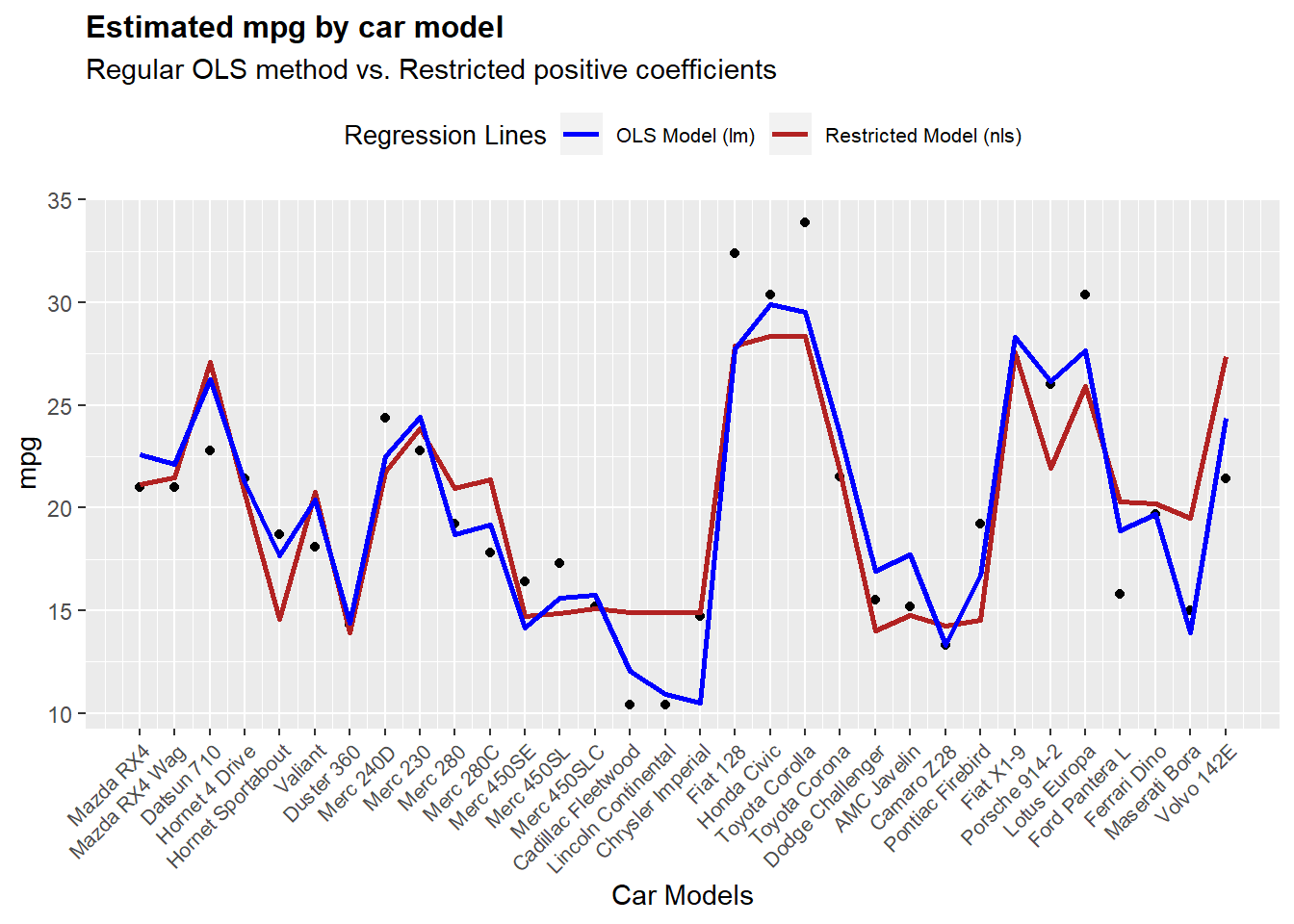
Let’s take a look at how each model predicts the output. Let’s keep in mind that we are predicting the response variable using the train set. This is, that all the cases that are used to train the model are the same we are using to compare accuracy. In this case we are going to omit this fact, but it is recommendable to keep a hold out set to compare both models fairly.
require(ggplot)
require(cowplot)
predict(fit3) -> pfit3
predict(fit4) -> pfit4

cols = c("Restricted Model (nls)" = "firebrick",
         "OLS Model (lm)" = "blue")
ggplot(mtcars,aes(x = 1:length(mpg),y = mpg)) +
  geom_point() +
  geom_line(aes(y = pfit3,colour = "Restricted Model (nls)"),size = 1) +
  geom_line(aes(y = pfit4,colour = "OLS Model (lm)"),size = 1) +
  scale_colour_manual(name="Regression Lines",values = cols) +
  scale_x_continuous(name = "Car Models",
                     breaks = 1:nrow(mtcars),
                     labels = row.names(mtcars)) +
    ggtitle(label = "Estimated mpg by car model",
            subtitle = "Regular OLS method vs. Restricted positive coefficients") +
  theme(axis.text.x = element_text(angle = 45, hjust = 1,size = 8),
        legend.position = "top",
        legend.text = element_text(size = 8),
        legend.title = element_text(size = 10),
plot.title = element_text(size = 12, face = "bold")) 
From this we can see that in terms of predictive power both models behave very similarly, and in practical terms both are going to give directionally similar answers. We can then use this result to estimate the impact of each one of these variables for the model.
Finally, a word of caution about the algorithm “Port”. Port comes from a library using nl2sol solution. In layman terms, tries to find lowest residual possible using something called nonlinear least-squares algorithm. As many other non-linear algorithms, the starting conditions could impact the results of the convergence. I personally recommend 3 approaches to lower the chances to encounter local minima.
Test different innitial conditions. By randomly picking different starting conditions we can evaluate if the results converge to similar coefficients.
Test cross validation. To evaluate the variance of the estimated coefficients.
Use alternative methods, such as Bayes and Lasso to see if all models reach the same conclusions.
