Forcing Regression Coefficients in R - Part II Lasso
Question:
I’m working on a regression model and I need to force the regression coefficients to be positive. How can I accomplish this in R?
Solution:
For linear model regression model with restricted coefficients you have 3 options: Linear with nls, Bayes with brms and Lasso. Here we will look at Linear Model with Lasso using glmnet
In this case glmnet provides a convenient way to restrict coefficients regularizing the coefficients. Here’s how to accomplish the question using R
if (!require(glmnet)) install.packages("glmnet")
if (!require(tidyverse)) install.packages("tidyverse")
# Install kable to visualize tables
if (!require(knitr)) install.packages("knitr")

# Store Independent variables into a Matrix
X <- model.matrix(Sepal.Length~.,data = iris)[,-1]

# Store dependent variable into a vector (in this case Sepal.Length)
y <- iris$Sepal.Length

# Choose Constrained Coefficients. In this case positive between 0 and Inf
lb <- rep(0,length(colnames( X )))
ub <- rep(Inf,length(colnames( X )))

# Now we have a 0 as lower bound for each variable in the model in the vector lb
# And we have a vector of Inf as upper bound for each variable in the model under ub

# Pick optimal lambda (this is optional as you can pick your own lambda)
cv.glmnet(x = X,y = y,
          lower.limits = lb,
          upper.limits = ub) -> cv_las1
cv_las1$lambda.min -> lambda

# Run glmnet (with min Lambda)
glmnet(x = X,y = y,
       lower.limits = lb,
       upper.limits = ub,
       lambda = lambda) -> las1

# See coefs
coef(las1) %>% as.matrix() %>% as.data.frame() -> c.fit1
colnames(c.fit1) <- c("Coefficient")

# See in a neat table
knitr::kable(c.fit1, caption = "Forced Positive Coefficients")| Coefficient | |
|---|---|
| (Intercept) | 2.4812335 |
| Sepal.Width | 0.5372833 |
| Petal.Length | 0.4575428 |
| Petal.Width | 0.0000000 |
| Speciesversicolor | 0.0000000 |
| Speciesvirginica | 0.0000000 |
Business Application
Glmnet is very useful when we are dealing with more columns than rows in our dataset. Lasso will shrink to 0, those coefficients that are not that useful compared to other variables.
I have used this approach for calculating price elasticity. This is because sometimes the data available to measure the fluctuation in price elasticity has a very short range of price points. With a small amount of data points we could easily overfit the data set and in turn get extreme values for Price point elasticities. Lasso can shrink these coefficients to more realistic values. We can even force Price to be part of the model by giving additional weight to the price variable. I provide an example of this below.
We have to consider that some variables can’t be used with the forced positive coefficient. It could be the case that no matter how we constraint the coefficient, the variable coefficient will quickly drop to 0. This is because the data is telling us the variable can’t really be positive.
In more detail
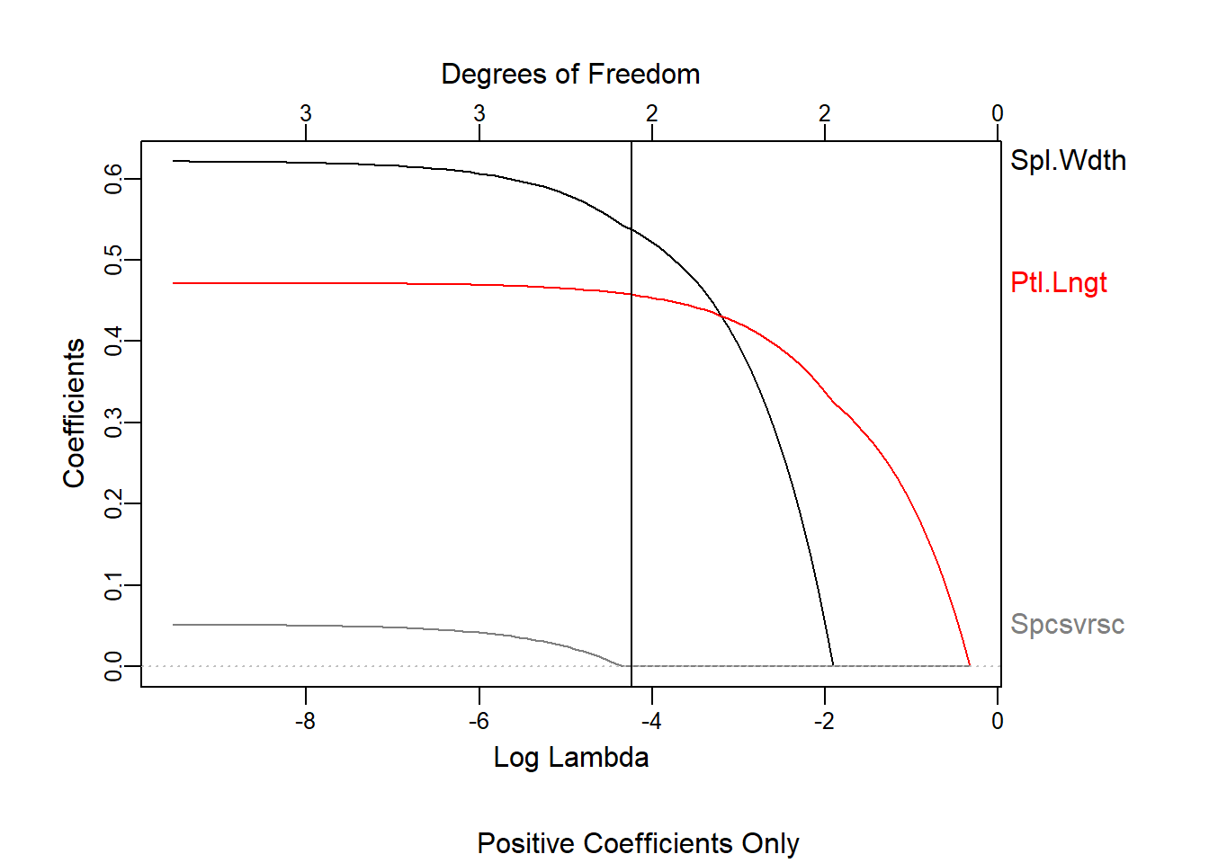
We can see what happened to the coefficients while the shrinkage process took place
if (!require(plotmo)) install.packages("plotmo")

glmnet(x = X,y = y,
       lower.limits = lb,
       upper.limits = ub) -> las2


plot_glmnet(las2,xvar = "lambda")
  title(sub = "Positive Coefficients Only")
abline(v = log(lambda))
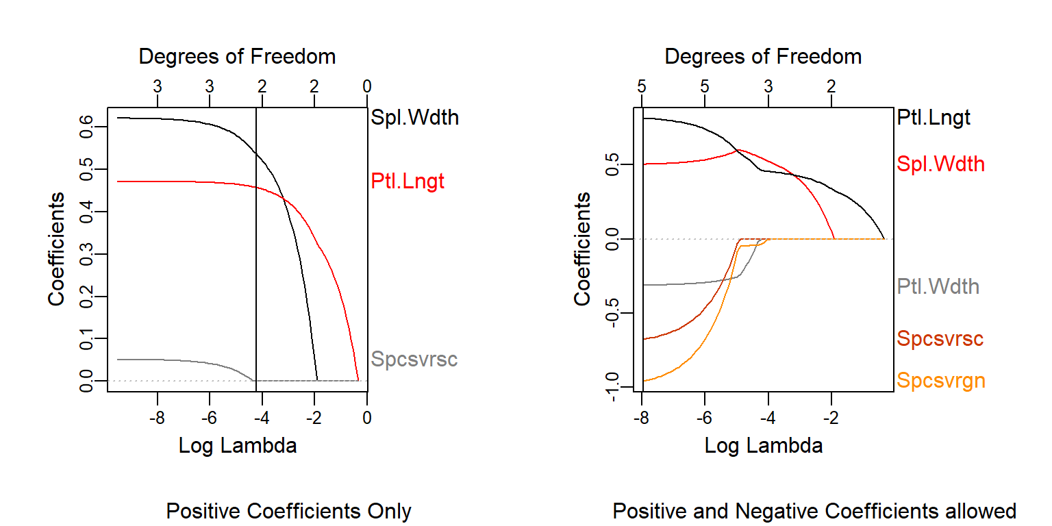
It’s very interesting to compare this to what would happen if we did not have any restriction in the coefs.
Let’s see them side by side
if (!require(plotmo)) install.packages("plotmo")

cv.glmnet(x = X,y = y) -> cv_las3
cv_las3$lambda.min -> lambda2

glmnet(x = X,y = y) -> las3

par(mfrow = c(1,2))

plot_glmnet(las2,xvar = "lambda")
  title(sub = "Positive Coefficients Only")
abline(v = log(lambda))

plot_glmnet(las3,xvar = "lambda")
  title(sub = "Positive and Negative Coefficients allowed")
abline(v = log(lambda2))
We see how Petal Width will not take positive coefficients even if we coerce the positive side of the values. This is because when we include Petal Length, the high correlation between the two variables makes it choose one for the upward relationship and the remaining one for the downward variance
# Save variables into y,x1,x2 to simplify formulas
iris$Sepal.Length -> y
iris$Petal.Length -> x1
iris$Petal.Width -> x2

# Regress y by each of the independent variables and each independent variable from each other
lm(y~x1) -> m1
lm(y~x2) -> m2
lm(x1~x2) -> m3
lm(x2~x1) -> m4

# Get the residuals with respect to each independent variable
resid(m1) -> r1
resid(m2) -> r2
resid(m3) -> r3
resid(m4) -> r4

par(mfrow = c(2,2),mar=c(2,2,2,2))

# Get the relationship between y and x1 (No other covariables)
plot(x1,y,pch = 20,col='grey',main = 'Sepal.Length ~ Petal.Length')
abline(m1,col = 'red')
text(x=2,y=7.5,labels =paste0("r = ",round(cor(y,x1),2)))

# Get the relationship between y and x2 (No other covariables)
plot(x2,y,pch = 20,col='grey',main = 'Sepal.Length ~ Petal.Width')
abline(m2,col = 'red')
text(x=0.5,y=7.5,labels =paste0("r = ",round(cor(y,x2),2)))

# Get residual correlation after factoring x2 from x1
plot(r1,r4,pch = 20,col='grey',main = 'Resid.Petal.Width ~ Resid.Petal.Length')
abline(lm(r4~r1),col = 'red')
text(x=-1,y=0.4,labels =paste0("r = ",round(cor(r1,r4),2)))


# Get residual correlation after factoring x1 from x2
plot(r2,r3,pch = 20,col='grey',main = 'Resid.Petal.Length ~ Resid.Petal.Width')
abline(lm(r3~r2),col = 'red')
text(x=-1,y=1,labels =paste0("r = ",round(cor(r2,r3),2)))
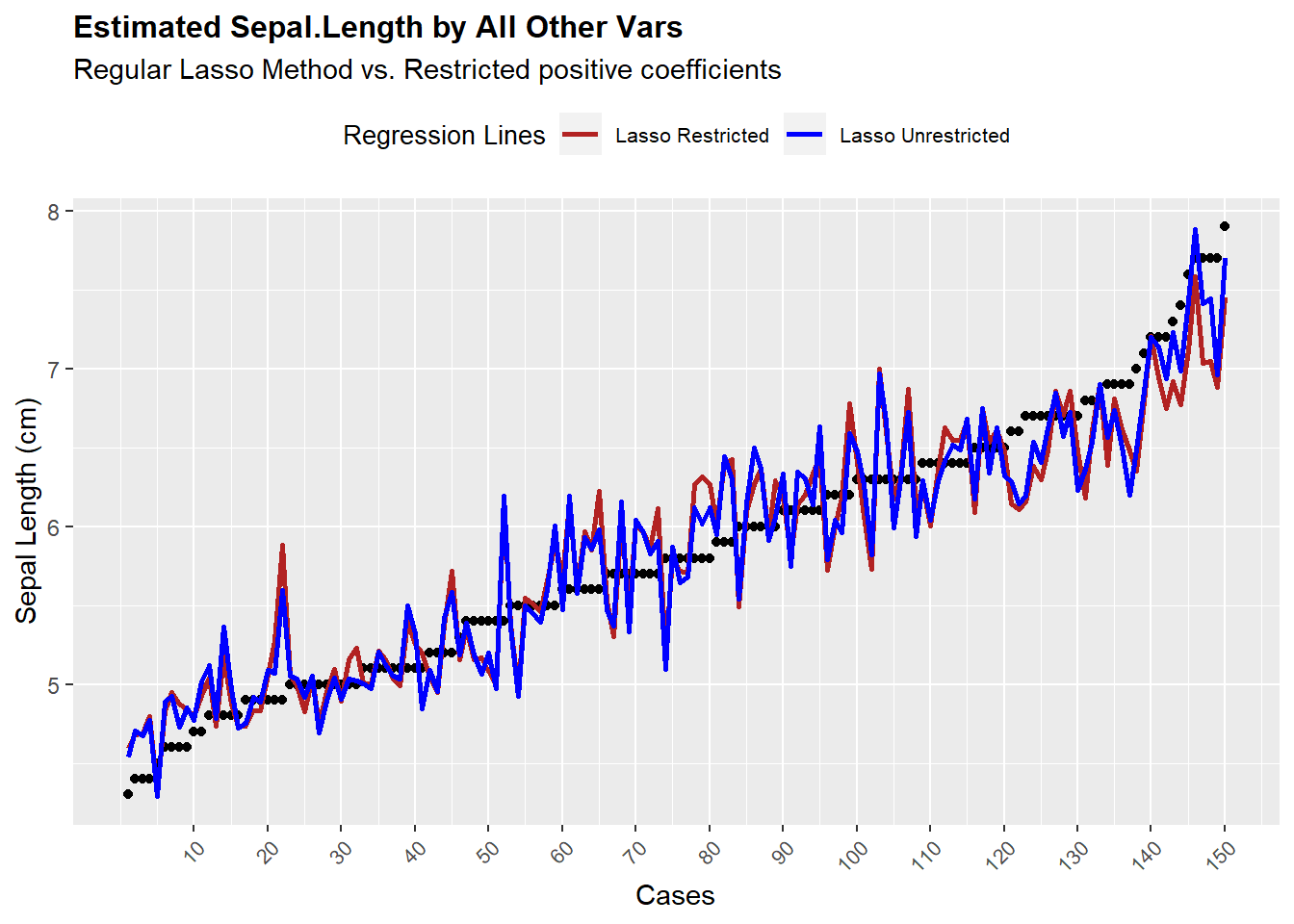
Now the last thing to test is to find out how good is the fit of this model compared to regular lm and unrestricted lasso model.
require(ggplot)
require(cowplot)
# Sort dependent and independent variables to visualize fit
y[order(y)] -> Yy
X[order(y),] -> Xy
predict(las1,s= lambda,newx = Xy) -> p1
predict(las3,s= lambda2,newx = Xy) -> p2
data.frame(Yy,p1= p1[,1],p2= p2[,1]) -> Z

cols = c("Lasso Restricted" = "firebrick",
         "Lasso Unrestricted" = "blue")

# Plot fits, blue is forced coefficients
ggplot(Z,aes(x = seq(1:length(Yy)),y = Yy)) +
  geom_point() +
  geom_line(aes(y = p1,colour = "Lasso Restricted"),size = 1) +
  geom_line(aes(y = p2,colour = "Lasso Unrestricted"),size = 1) +
  ylab("Sepal Length (cm)") +
  scale_colour_manual(name="Regression Lines",values = cols) +
  scale_x_continuous(name = "Cases",
                     breaks = seq(10,150,by = 10)) +
    ggtitle(label = "Estimated Sepal.Length by All Other Vars",
            subtitle = "Regular Lasso Method vs. Restricted positive coefficients") +
  theme(axis.text.x = element_text(angle = 45, hjust = 1,size = 8),
        legend.position = "top",
        legend.text = element_text(size = 8),
        legend.title = element_text(size = 10),
plot.title = element_text(size = 12, face = "bold")) 
We see the model is somewhat erratic, but on average it fits the data well, except for the extreme cases of the dependent variable. But the main concept we should keep in mind is that both models perform similarly at fitting the data points.
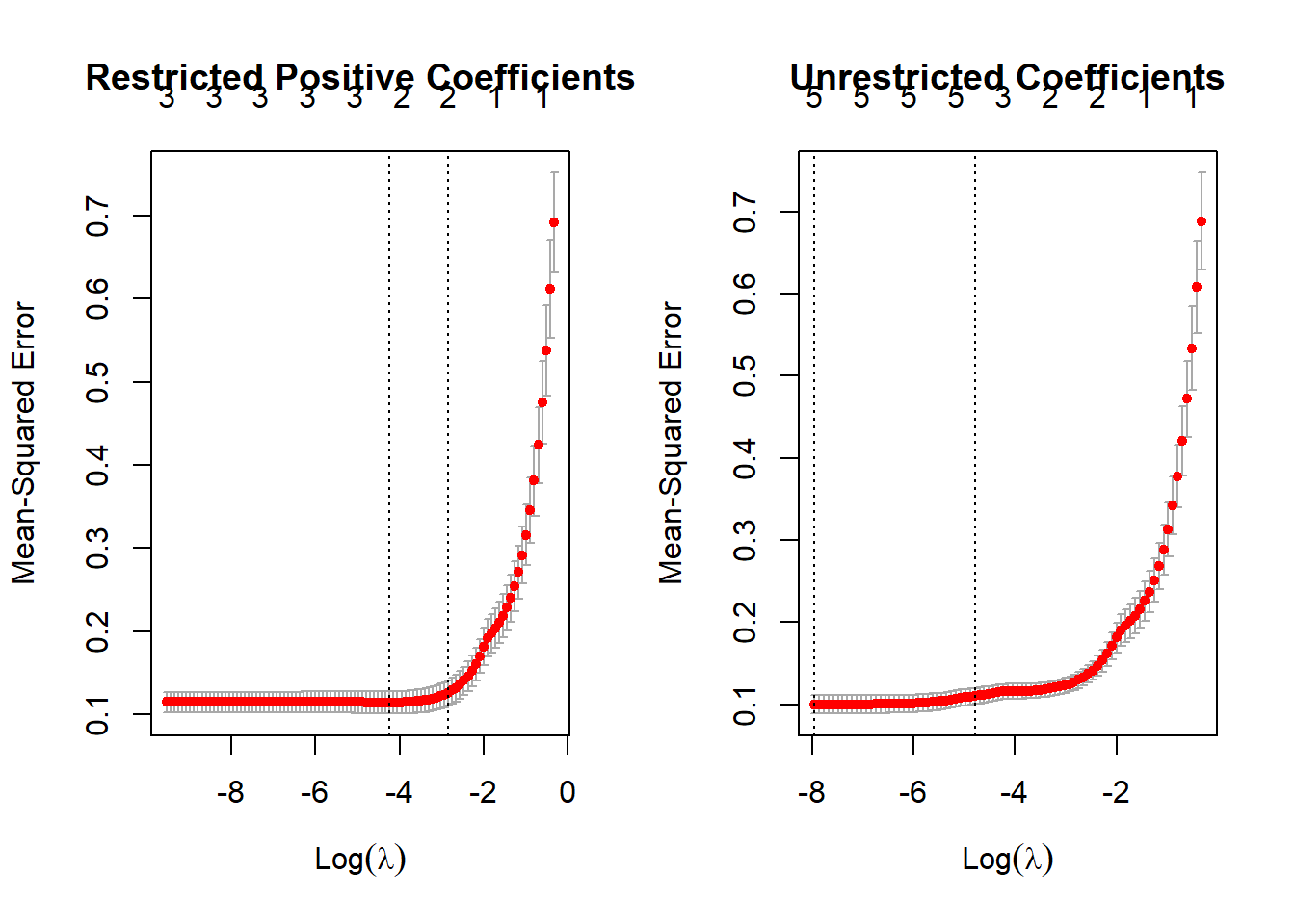
We would have to now assess if the model is good when predicting Cross Validated data which the model in lasso allows to look.
par(mfrow=c(1,2))
plot(cv_las1,main = "Restricted Positive Coefficients")
plot(cv_las3, main = "Unrestricted Coefficients")
And as we see the restricted model has a Mean-squared error out-of sample of 0.115 while the unrestricted model has an error of 0.1, which is not a big difference and even we could say is more parsimonious in terms of number of variables.
