Tutorial:How does certainty of beta estimation changes with sample size?
Linear Regression
We first simulate data to see how to see how to calculate beta (slope) and alpha (constant) coefficients. We use a sampling method from a multivariate normal distribution with mean [0,0] and some covariance between independent variable x and target variable y.
# Import Libraries
import numpy as np
import matplotlib.pyplot as plt

m = range(0,10000) # Datasets
n = 100 # number of points
sigx = .3 # Standard deviation x
sigy = .9 # Standard deviation y
rho = .1 # Pearson rho correlation used to show level of linear dependence

# generate data
mu = np.array([0.,0.])
cov = np.array([[sigx*sigx,rho*sigx*sigy],[rho*sigx*sigy,sigy*sigy]])

data = np.random.multivariate_normal(mu,cov,n) # Sample data

x = data[:,0]
y = data[:,1]

# fit the model
covmat = np.cov(x,y) # covariance matrix
# cov of x,y is also estimated as rho(x,y)*sigma(x)*sigma(y)

# best fit parameters
betahat = covmat[0,1]/covmat[0,0] # covariance x,y divided by variance x
alphahat = np.mean(y) - betahat*np.mean(x)

# plot best fit model
xvals = np.linspace(-1,1,150)
yvals = betahat*xvals + alphahat

# Plot distribution density map
plt.figure()
plt.hist2d(x,y)
## (array([[0., 0., 3., 0., 0., 1., 0., 0., 0., 0.],
## [0., 0., 1., 0., 0., 0., 1., 0., 0., 0.],
## [0., 1., 0., 0., 2., 1., 1., 1., 0., 0.],
## [0., 0., 0., 1., 2., 0., 1., 2., 0., 0.],
## [0., 0., 3., 6., 3., 2., 1., 0., 0., 1.],
## [2., 1., 6., 2., 1., 3., 4., 0., 2., 0.],
## [0., 0., 3., 3., 2., 2., 1., 2., 2., 0.],
## [0., 0., 0., 2., 1., 0., 1., 3., 1., 1.],
## [0., 1., 0., 1., 4., 3., 2., 0., 3., 0.],
## [0., 0., 1., 0., 1., 1., 3., 0., 1., 0.]]), array([-0.75887284, -0.62767179, -0.49647074, -0.36526969, -0.23406864,
## -0.1028676 , 0.02833345, 0.1595345 , 0.29073555, 0.4219366 ,
## 0.55313765]), array([-1.73772901, -1.3580218 , -0.9783146 , -0.5986074 , -0.2189002 ,
## 0.16080701, 0.54051421, 0.92022141, 1.29992862, 1.67963582,
## 2.05934302]), <matplotlib.collections.QuadMesh object at 0x000000002EAA8E80>)plt.show()
# Plot data points + Regression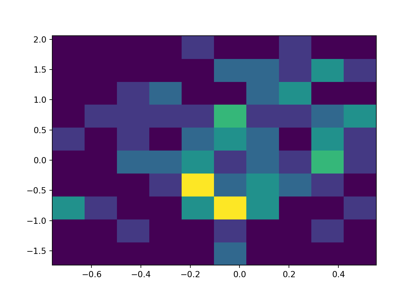
plt.figure()
plt.plot(x,y,'bx')
plt.plot(xvals,yvals,'r-')
plt.show()

Problem 1:
Plot histogram of these values and comment on its shape. How does this histogram change as you change n and rho? Interpret the results
Let’s first define a function that takes the innitial inputs and calculates beta several (m) times. We then store this list of betas to analyze the effect of changing n and rho.
def betas(sigx,sigy,rho,n,m):
  """function to calculate beta m times by sampling from normal distribution.
  Function takes boolean inputs, returns list"""
  betas = [] # Store results
  mu = np.array([0.,0.])
  cov = np.array([[ sigx*sigx , rho*sigx*sigy ],[ rho*sigx*sigy , sigy*sigy]])
  for i in m:
    # LOOP over
    # Sample the data with mu and covariance matrix
    data = np.random.multivariate_normal(mu,cov,n)
    x = data[:,0]
    y = data[:,1]
    # fit the model
    covmat = np.cov(x,y) # covariance matrix of x and y
    betahat = covmat[0,1]/covmat[0,0] # Covmat[0,1] is the first row of the matrix covmat, 2nd column. And its the covariance of x,y, covmat[0,0] is the quasivariance of x
    alphahat = np.mean(y) - betahat*np.mean(x) #alphahat is the mean value of y - meanvalue of x times the slope.
    # When x,y relationship is 1 to 1 then constant is the distance between average y and average x (scaling both axis to common origin, the constant)
    # Save beta in vector
    betas.append(betahat)
    # plot best fit model
    xvals = np.linspace(-1,1,150) # line of points where to calculate values
    yvals = betahat*xvals + alphahat

  return(betas)
Now that we have the function let’s visualize what happens when we use large n vs small n sample size.
# small n vs big n
n = 50
small_n = betas(sigx,sigy,rho,n,m)

n = 1000
big_n = betas(sigx,sigy,rho,n,m)

# Plot comparison for a small sample n vs big sample n
plt.figure()
plt.hist(small_n, bins = 30, color = 'blue')
## (array([2.000e+00, 1.000e+00, 1.000e+00, 7.000e+00, 1.200e+01, 3.000e+01,
## 6.300e+01, 1.050e+02, 1.530e+02, 2.740e+02, 4.420e+02, 5.800e+02,
## 8.690e+02, 9.910e+02, 1.127e+03, 1.170e+03, 1.046e+03, 9.740e+02,
## 7.200e+02, 5.130e+02, 4.180e+02, 2.050e+02, 1.400e+02, 7.400e+01,
## 4.700e+01, 2.200e+01, 8.000e+00, 3.000e+00, 1.000e+00, 2.000e+00]), array([-1.59794844, -1.47400642, -1.3500644 , -1.22612237, -1.10218035,
## -0.97823833, -0.85429631, -0.73035428, -0.60641226, -0.48247024,
## -0.35852821, -0.23458619, -0.11064417, 0.01329785, 0.13723988,
## 0.2611819 , 0.38512392, 0.50906595, 0.63300797, 0.75694999,
## 0.88089201, 1.00483404, 1.12877606, 1.25271808, 1.37666011,
## 1.50060213, 1.62454415, 1.74848618, 1.8724282 , 1.99637022,
## 2.12031224]), <a list of 30 Patch objects>)plt.hist(big_n, bins = 30, color = 'red')## (array([1.000e+00, 3.000e+00, 2.000e+00, 6.000e+00, 1.700e+01, 2.400e+01,
## 5.200e+01, 8.800e+01, 1.560e+02, 2.390e+02, 3.860e+02, 5.340e+02,
## 7.290e+02, 8.590e+02, 1.010e+03, 1.058e+03, 9.760e+02, 9.900e+02,
## 8.170e+02, 6.420e+02, 5.330e+02, 3.510e+02, 2.200e+02, 1.490e+02,
## 6.800e+01, 5.100e+01, 2.300e+01, 1.300e+01, 1.000e+00, 2.000e+00]), array([-0.09540655, -0.07056651, -0.04572647, -0.02088643, 0.00395362,
## 0.02879366, 0.0536337 , 0.07847374, 0.10331378, 0.12815382,
## 0.15299386, 0.17783391, 0.20267395, 0.22751399, 0.25235403,
## 0.27719407, 0.30203411, 0.32687415, 0.35171419, 0.37655424,
## 0.40139428, 0.42623432, 0.45107436, 0.4759144 , 0.50075444,
## 0.52559448, 0.55043453, 0.57527457, 0.60011461, 0.62495465,
## 0.64979469]), <a list of 30 Patch objects>)plt.show()
In blue we see how a small n makes the uncertainty around the beta greater. It makes the number oscillate between 1 and 3. While when our sampling size is greater our potential betas are more concentrated around the mean. See the differences between the means and the standard deviations
# print means for both groups
np.mean(small_n)
## 0.2981638939327568np.mean(big_n)
# print Std for both groups ## 0.2990726218301166np.std(small_n)## 0.4372268184404137np.std(big_n)## 0.09420414145370962Now let’s do the same for a large value of rho and and a small effect closer to 0.
# Small Rho vs big Rho
n = 100 # adjust again n

# Small Rho
rho = 0.01
small_rho = betas(sigx,sigy,rho,n,m)

# Big Rho
rho = 0.9
big_rho = betas(sigx,sigy,rho,n,m)

# Plot comparison for a small rho n vs big rho
plt.figure()
plt.hist(small_rho, bins = 30, color = 'blue')
## (array([2.000e+00, 0.000e+00, 2.000e+00, 1.300e+01, 1.300e+01, 3.700e+01,
## 6.900e+01, 1.100e+02, 1.860e+02, 3.010e+02, 4.720e+02, 6.800e+02,
## 8.120e+02, 9.840e+02, 1.032e+03, 1.117e+03, 1.022e+03, 9.300e+02,
## 7.240e+02, 5.500e+02, 3.860e+02, 2.540e+02, 1.420e+02, 7.600e+01,
## 4.600e+01, 2.500e+01, 6.000e+00, 7.000e+00, 1.000e+00, 1.000e+00]), array([-1.24139818, -1.15807321, -1.07474823, -0.99142326, -0.90809828,
## -0.82477331, -0.74144834, -0.65812336, -0.57479839, -0.49147341,
## -0.40814844, -0.32482347, -0.24149849, -0.15817352, -0.07484854,
## 0.00847643, 0.09180141, 0.17512638, 0.25845135, 0.34177633,
## 0.4251013 , 0.50842628, 0.59175125, 0.67507622, 0.7584012 ,
## 0.84172617, 0.92505115, 1.00837612, 1.09170109, 1.17502607,
## 1.25835104]), <a list of 30 Patch objects>)plt.hist(big_rho, bins = 30, color = 'red')## (array([1.000e+00, 0.000e+00, 2.000e+00, 4.000e+00, 1.000e+01, 1.500e+01,
## 4.500e+01, 8.100e+01, 1.690e+02, 2.650e+02, 3.860e+02, 5.460e+02,
## 7.230e+02, 9.080e+02, 1.125e+03, 1.111e+03, 1.090e+03, 9.760e+02,
## 8.130e+02, 5.940e+02, 4.540e+02, 2.940e+02, 1.800e+02, 1.050e+02,
## 6.400e+01, 2.300e+01, 1.100e+01, 3.000e+00, 1.000e+00, 1.000e+00]), array([2.11639398, 2.15367914, 2.1909643 , 2.22824946, 2.26553461,
## 2.30281977, 2.34010493, 2.37739009, 2.41467525, 2.45196041,
## 2.48924556, 2.52653072, 2.56381588, 2.60110104, 2.6383862 ,
## 2.67567136, 2.71295652, 2.75024167, 2.78752683, 2.82481199,
## 2.86209715, 2.89938231, 2.93666747, 2.97395263, 3.01123778,
## 3.04852294, 3.0858081 , 3.12309326, 3.16037842, 3.19766358,
## 3.23494873]), <a list of 30 Patch objects>)plt.show()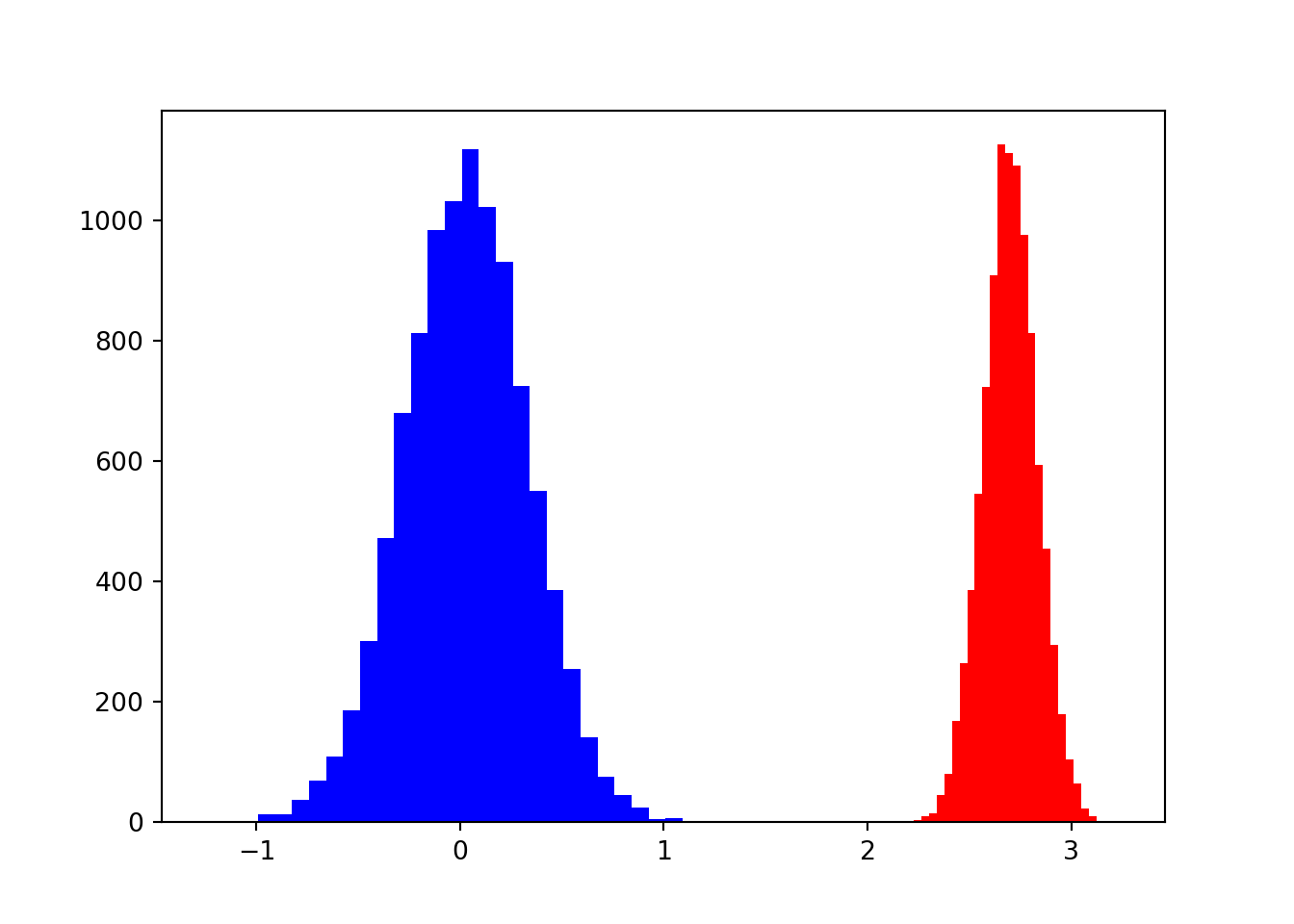
In this case we see how rho affects at the correlation between x and y. When rho is small the values of beta are more likely to be zero. On the other hand, when rho is high values of beta are extremely different from 0
Problem 2:
Implement the standard error formula for betahat. Extend your work in the prior problem to compute the normalized coefficient zhat = betahat/std(betahat). Look into scipy.stats package and find the student-t distribution. Use the t.pdf() function to plot a student-t distribution with v = n - 2 degrees of freedom on top of a histogram of zhat values and compare the two.
For this we will first implement a standard error formula for betahat. This function is defined as we saw in class as
# Define the Standard Error formula
def se_beta(y,x,df):
  # An estimate for se(betahat) = sqrt((1/v sum(yhat - yi)^2)/sum(xi-mean(x)^2))

  # define degrees of freedom t distribution
  v = 1/df

  # define y hat from the beta value
  yhat = alphahat + betahat*x # estimate yhat
  # Calculate standard error of betahat
  # Calculate numerator and denominator
  num = v * np.sum((yhat - y)**2) # sum of squared error of predicted yhat
  dem = np.sum((x - np.mean(x))**2) # Var of x

  # return se_beta: how much does yhat err scaled by the variance of x
  return(np.sqrt(num/dem))


# Include this in the function we created previously and store zhat of every iteration

def zetas(sigx,sigy,rho,n,m):
  """docstring for betas"""
  zetas = [] # Store results
  mu = np.array([0.,0.])
  cov = np.array([[ sigx*sigx , rho*sigx*sigy ],[ rho*sigx*sigy , sigy*sigy]])
  for i in m:
    # LOOP over
    # Sample the data with mu and covariance matrix
    data = np.random.multivariate_normal(mu,cov,n)
    x = data[:,0]
    y = data[:,1]

    # fit the model
    covmat = np.cov(x,y) # covariance matrix of x and y
    betahat = covmat[0,1]/covmat[0,0] # Covmat[0,1] is the first row of the matrix covmat, 2nd column. And its the covariance of x,y, covmat[0,0] is the quasivariance of x
    alphahat = np.mean(y) - betahat*np.mean(x) #alphahat is the mean value of y - meanvalue of x times the slope.

    # Calculate Standard Error and zhat
    se_betahat = se_beta(y,x,df = (n-2))
    zhat = (betahat / se_betahat)
    # Save zeta in vector
    zetas.append(zhat)

  return(zetas)


# Create t distribution line rv, and probability (pdf)
from scipy.stats import t
rv = t(df=(n - 2), loc=0, scale=1)
# plot best fit model
xvals = np.linspace(-4,4,150) # line of points where to calculate values
yvals = betahat*xvals + alphahat
Now that we can calculate the standard error of beta we can calculate the z-score and compare that to the theoretical t-student distribution around value 0. We can visually see if one is different from the other.
# rho high
rho = 0.7
zeta_hats = zetas(sigx,sigy,rho,n,m)

# Compare t-distribution with v degrees of freedom (blue) and actual zhat distribution when rho is high (orange)
plt.figure()
plt.plot(xvals,rv.pdf(x=xvals))
plt.hist(zeta_hats,density = True,histtype = 'stepfilled',bins = 50)
## (array([0.00081189, 0. , 0. , 0. , 0.00081189,
## 0.00324758, 0.00081189, 0.00081189, 0.00162379, 0.00324758,
## 0.00162379, 0.00893084, 0.015426 , 0.01786169, 0.0162379 ,
## 0.02922822, 0.04627801, 0.06251591, 0.07469433, 0.12097234,
## 0.12827939, 0.18348824, 0.20378561, 0.24032088, 0.28822268,
## 0.36210511, 0.42218534, 0.48145366, 0.50012724, 0.49363208,
## 0.54234578, 0.56507883, 0.55614799, 0.48388935, 0.44897787,
## 0.40026417, 0.39458091, 0.29552973, 0.20216182, 0.17212171,
## 0.12990318, 0.09417981, 0.06008022, 0.02192116, 0.02110927,
## 0.01299032, 0.00405947, 0.00243568, 0.00162379, 0.00081189]), array([ 4.17437087, 4.29753953, 4.42070818, 4.54387684, 4.66704549,
## 4.79021415, 4.9133828 , 5.03655146, 5.15972011, 5.28288877,
## 5.40605742, 5.52922608, 5.65239473, 5.77556339, 5.89873204,
## 6.0219007 , 6.14506935, 6.26823801, 6.39140666, 6.51457532,
## 6.63774397, 6.76091263, 6.88408129, 7.00724994, 7.1304186 ,
## 7.25358725, 7.37675591, 7.49992456, 7.62309322, 7.74626187,
## 7.86943053, 7.99259918, 8.11576784, 8.23893649, 8.36210515,
## 8.4852738 , 8.60844246, 8.73161111, 8.85477977, 8.97794842,
## 9.10111708, 9.22428573, 9.34745439, 9.47062304, 9.5937917 ,
## 9.71696035, 9.84012901, 9.96329766, 10.08646632, 10.20963498,
## 10.33280363]), <a list of 1 Patch objects>)plt.show()
# rho small (small beta)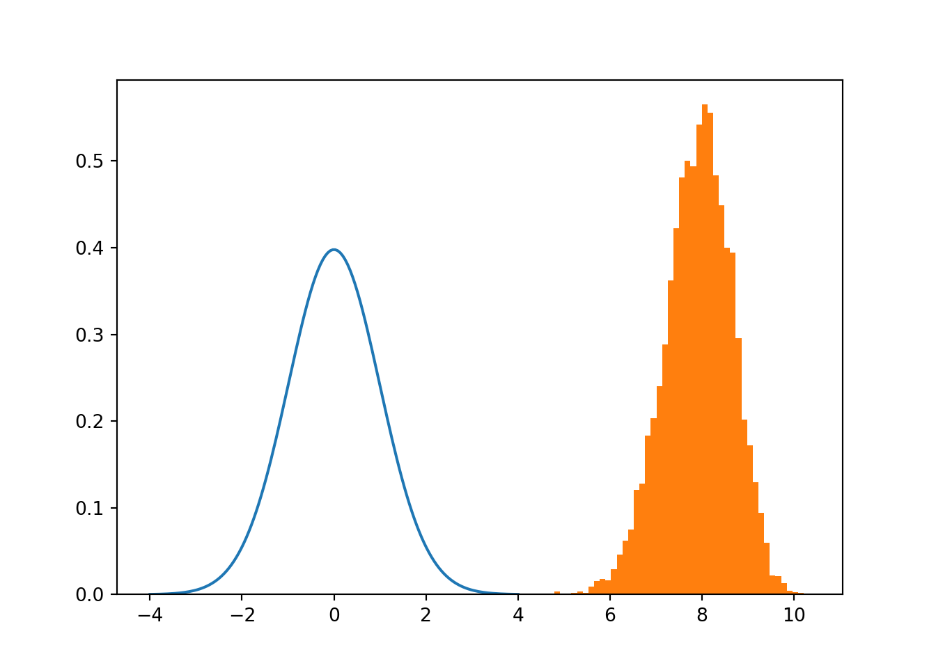
rho = 0.01
zeta_hats = zetas(sigx,sigy,rho,n,m)

# Compare t-distribution with v degrees of freedom (blue) and actual zhat distribution when rho is low (orange)
plt.figure()
plt.plot(xvals,rv.pdf(x=xvals))
plt.hist(zeta_hats,density = True,histtype = 'stepfilled',bins = 50)
## (array([0.0013281 , 0.00066405, 0.0013281 , 0.00531241, 0.00664052,
## 0.01128888, 0.01527319, 0.02523397, 0.03785095, 0.04382742,
## 0.07171759, 0.08898294, 0.11620906, 0.15870837, 0.19323906,
## 0.22378544, 0.26628475, 0.30812002, 0.34995528, 0.35194743,
## 0.37983761, 0.397767 , 0.40971993, 0.42300097, 0.40639968,
## 0.37120493, 0.33202588, 0.3220651 , 0.26362855, 0.2065201 ,
## 0.19655932, 0.14542733, 0.12550578, 0.0949594 , 0.09031104,
## 0.06640518, 0.04449147, 0.02191371, 0.02456992, 0.01593724,
## 0.00929672, 0.00464836, 0.00199216, 0.00332026, 0.00265621,
## 0.00066405, 0.0013281 , 0. , 0. , 0.00066405]), array([-3.29630691, -3.14571624, -2.99512557, -2.8445349 , -2.69394422,
## -2.54335355, -2.39276288, -2.24217221, -2.09158154, -1.94099087,
## -1.79040019, -1.63980952, -1.48921885, -1.33862818, -1.18803751,
## -1.03744684, -0.88685617, -0.73626549, -0.58567482, -0.43508415,
## -0.28449348, -0.13390281, 0.01668786, 0.16727853, 0.31786921,
## 0.46845988, 0.61905055, 0.76964122, 0.92023189, 1.07082256,
## 1.22141323, 1.37200391, 1.52259458, 1.67318525, 1.82377592,
## 1.97436659, 2.12495726, 2.27554794, 2.42613861, 2.57672928,
## 2.72731995, 2.87791062, 3.02850129, 3.17909196, 3.32968264,
## 3.48027331, 3.63086398, 3.78145465, 3.93204532, 4.08263599,
## 4.23322666]), <a list of 1 Patch objects>)plt.show()
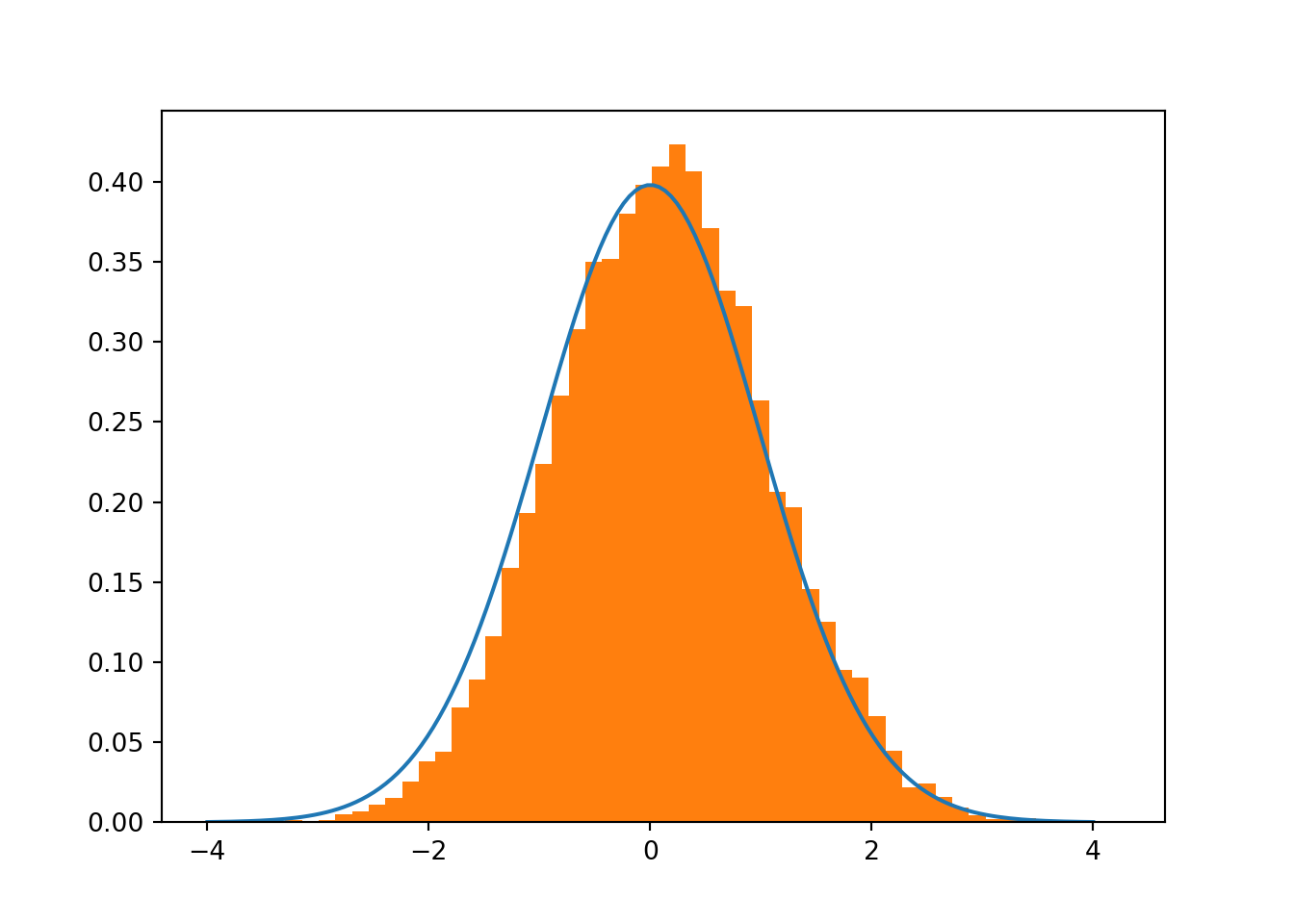
When beta coefficient is high there’s a high probability the value is different than 0 empirical sampling shows little to no overlap when rho is high, basically discarding the hypothesis that beta = 0 However, overlap seems significant when rho is close to 0.
Problem 3:
Implement the p-value formula we mentioned in class using the quad method in scipy.integrate, and the student-t distribution from the prior problem Next, consider the OLS method in statsmodels. Fit a dataset using both methods that we considered in class and statmodels methods. Compute the summary stats of the statsmodels method, which includes betahat errors as well as associated p-values with your results from Problem 2
# P-value formula using scipy.integrate

import scipy.integrate as Int
rho = 0.3
mu = np.array([0.,0.])
cov = np.array([[ sigx*sigx , rho*sigx*sigy ],[ rho*sigx*sigy , sigy*sigy]])
data = np.random.multivariate_normal(mu,cov,n)
x = data[:,0]
y = data[:,1]

# fit the model
covmat = np.cov(x,y) # covariance matrix of x and y
betahat = covmat[0,1]/covmat[0,0] # Covmat[0,1] is the first row of the matrix covmat, 2nd column. And its the covariance of x,y, covmat[0,0] is the quasivariance of x
alphahat = np.mean(y) - betahat*np.mean(x) #alphahat is the mean value of y - meanvalue of x times the slope.

# Calculate Standard Error and zhat
se_betahat = se_beta(y,x,df = (n-2))
zhat = (betahat / se_betahat)


pvalue_integration = Int.quad(rv.pdf,zhat,np.inf)[0]*2

# Check with OLS method
import statsmodels.api as sm
# help(sm.OLS)
X = sm.add_constant(x)
model = sm.OLS(y,X).fit()
model.summary()
## <class 'statsmodels.iolib.summary.Summary'>
## """
## OLS Regression Results
## ==============================================================================
## Dep. Variable: y R-squared: 0.081
## Model: OLS Adj. R-squared: 0.071
## Method: Least Squares F-statistic: 8.607
## Date: Thu, 26 Mar 2020 Prob (F-statistic): 0.00417
## Time: 18:01:16 Log-Likelihood: -124.78
## No. Observations: 100 AIC: 253.6
## Df Residuals: 98 BIC: 258.8
## Df Model: 1
## Covariance Type: nonrobust
## ==============================================================================
## coef std err t P>|t| [0.025 0.975]
## ------------------------------------------------------------------------------
## const -0.0965 0.087 -1.115 0.268 -0.268 0.075
## x1 0.8428 0.287 2.934 0.004 0.273 1.413
## ==============================================================================
## Omnibus: 0.823 Durbin-Watson: 2.212
## Prob(Omnibus): 0.663 Jarque-Bera (JB): 0.866
## Skew: -0.068 Prob(JB): 0.649
## Kurtosis: 2.565 Cond. No. 3.39
## ==============================================================================
##
## Warnings:
## [1] Standard Errors assume that the covariance matrix of the errors is correctly specified.
## """pvalue_OLS = model.pvalues[1]
# plot distribution and z score
plt.figure()
plt.plot(xvals,rv.pdf(xvals))
plt.vlines(zhat,0,0.5)
plt.show()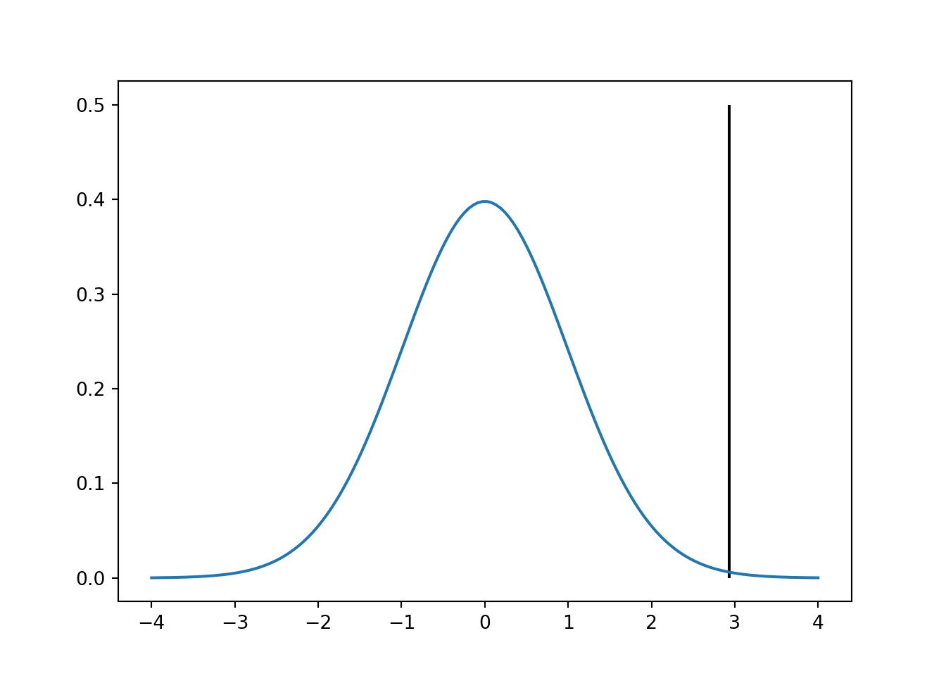
We can visually see that the z-score value is far from the mean. Now we can calculate the probability that the value is different from zero. In this case we are going to compare the 2 methods we used.
# P-value via integration
print('-------- P-value via integration -----------')
## -------- P-value via integration -----------print(pvalue_integration)
# P-value via statsmodels package ## 0.004170110594249354print('-------- P-value via statsmodels package -----------')## -------- P-value via statsmodels package -----------print(pvalue_OLS)
## 0.004170110594249177As we can see both p-values are exactly the same when we calculate them via integration or with the statsmodel package
