How to fit sigmoid to time series data
Question:
How can I fit a sigmoid function to time series data in R? Because when I run nls I get the following error Error in nlsModel(formula, mf, start, wts) : singular gradient matrix at initial parameter estimates
Solution:
Normally we find many problems when trying to fit a non linear model to time series data. Specifically, when we don’t define correctly the starting values we get the error of singular gradient matrix error. The fact that every value of time corresponds to only one value on the y-axis makes the whole process harder for the solver in R. The solution is to use Self Start models
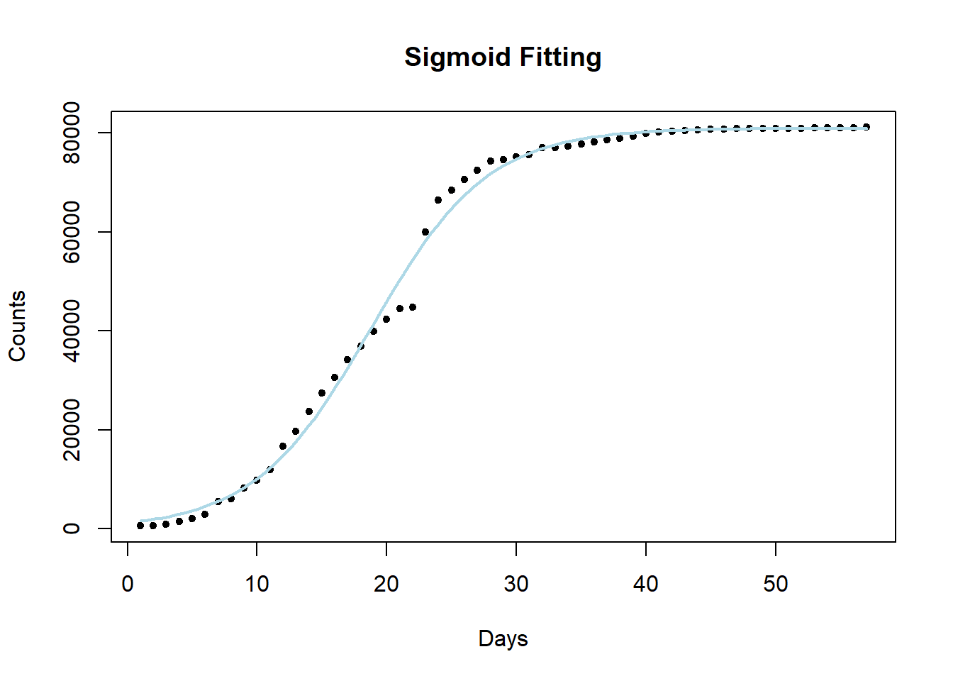
To fit a non linear regression with a sigmoid function to time series data you can use the nls function with a self-start function. In this case SSlogis
require(tidyverse)

# Create data set
tbl <- tibble::tribble(~date,~y,  "2020-01-22",   548L,  "2020-01-23",   643L,  "2020-01-24",   920L,  "2020-01-25",  1406L,  "2020-01-26",  2075L,  "2020-01-27",  2877L,  "2020-01-28",  5509L,  "2020-01-29",  6087L,  "2020-01-30",  8141L,  "2020-01-31",  9802L,  "2020-02-01", 11891L,  "2020-02-02", 16630L,  "2020-02-03", 19716L,  "2020-02-04", 23707L,  "2020-02-05", 27440L,  "2020-02-06", 30587L,  "2020-02-07", 34110L,  "2020-02-08", 36814L,  "2020-02-09", 39829L,  "2020-02-10", 42354L,  "2020-02-11", 44386L,  "2020-02-12", 44759L,  "2020-02-13", 59895L,  "2020-02-14", 66358L,  "2020-02-15", 68413L,  "2020-02-16", 70513L,  "2020-02-17", 72434L,  "2020-02-18", 74211L,  "2020-02-19", 74619L,  "2020-02-20", 75077L,  "2020-02-21", 75550L,  "2020-02-22", 77001L,  "2020-02-23", 77022L,  "2020-02-24", 77241L,  "2020-02-25", 77754L,  "2020-02-26", 78166L,  "2020-02-27", 78600L,  "2020-02-28", 78928L,  "2020-02-29", 79356L,  "2020-03-01", 79932L,  "2020-03-02", 80136L,  "2020-03-03", 80261L,  "2020-03-04", 80386L,  "2020-03-05", 80537L,  "2020-03-06", 80690L,  "2020-03-07", 80770L,  "2020-03-08", 80823L,  "2020-03-09", 80860L,  "2020-03-10", 80887L,  "2020-03-11", 80921L,  "2020-03-12", 80932L,  "2020-03-13", 80945L,  "2020-03-14", 80977L,  "2020-03-15", 81003L,  "2020-03-16", 81033L,  "2020-03-17", 81058L,  "2020-03-18", 81102L)

# Convert Date to Sequence (Because you can't regress dates)
tbl <- tbl %>% mutate(x = seq_along(tbl$date))

# Run regression nls with formula SSlogis both from package stats
fit <- nls(y ~ SSlogis(x, a, b, c), data = tbl)

# Check model
summary(fit)
##
## Formula: y ~ SSlogis(x, a, b, c)
##
## Parameters:
## Estimate Std. Error t value Pr(>|t|)
## a 8.093e+04 4.640e+02 174.4 <2e-16 ***
## b 1.876e+01 1.604e-01 116.9 <2e-16 ***
## c 4.503e+00 1.385e-01 32.5 <2e-16 ***
## ---
## Signif. codes: 0 '***' 0.001 '**' 0.01 '*' 0.05 '.' 0.1 ' ' 1
##
## Residual standard error: 2188 on 54 degrees of freedom
##
## Number of iterations to convergence: 0
## Achieved convergence tolerance: 3.639e-06# Save coefficients
p <- coef(fit)
# Plot output
attach(tbl)
plot(x,y,title(main = "Sigmoid Fitting"),xlab = "Days",ylab = 'Counts',pch = 20)
curve(SSlogis(x,p["a"],p["b"],p["c"]),lwd = 2, col = 'lightblue',add = TRUE) # Predict
detach(tbl)That’s it that’s all you need
Additional stuff
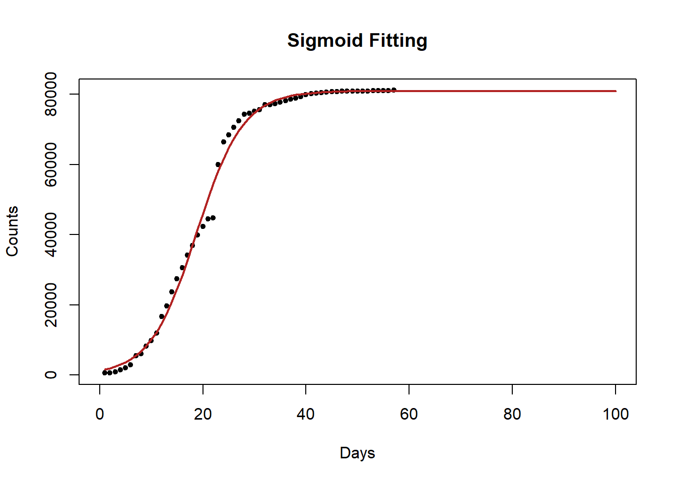
We can also project our model further out
# Plot data again
attach(tbl)
plot(x,y,title(main = "Sigmoid Fitting"),xlab = "Days",ylab = 'Counts',pch = 20,xlim = c(0,100))
detach(tbl)

# Plot further out output
new_x <- seq(1,100)
lines(SSlogis(new_x,p["a"],p["b"],p["c"]),lwd = 2, col = 'firebrick') # Predict
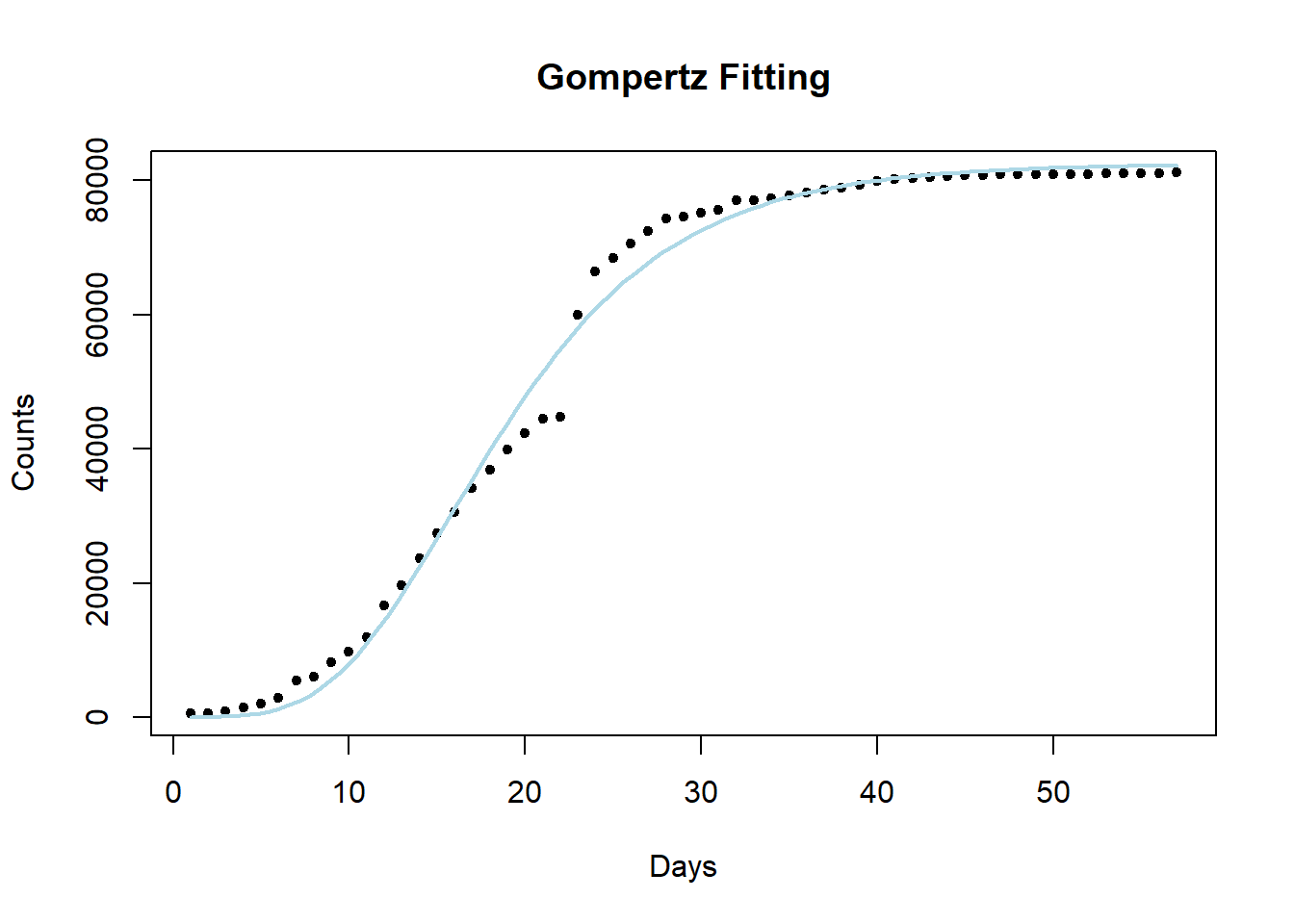
You can use a different function to fit this too. There’s a long list of Self starting Non linear
# Fit an assymptotic curve SSgompertz(x, Asym, b2, b3)
# Run regression nls with formula SSlogis both from package stats
fit_gompertz <- nls(y ~ SSgompertz(x, a, b, c), data = tbl)

# Check model
# summary(fit_gompertz)

# Save coefficients
p <- coef(fit_gompertz)

# Plot output
attach(tbl)
plot(x,y,title(main = "Gompertz Fitting"),xlab = "Days",ylab = 'Counts',pch = 20)
curve(SSgompertz(x,p["a"],p["b"],p["c"]),lwd = 2, col = 'lightblue',add = TRUE) # Predict
detach(tbl)You can also calculate a model R-square by fitting this curve to a linear model
require(broom)
# Regress both non-linear outputs in a linear model to get R-squares
lm(y~predict(fit),data = tbl)  -> lmfit_logistic
lm(y~predict(fit_gompertz),data = tbl) -> lmfit_gompertz


# Comparing R-squares
Comparison <- data.frame(
Regression = c("Logistic","Gompertz"),
RSquare = c(summary(lmfit_logistic)$r.squared ,summary(lmfit_gompertz)$r.squared))

Comparison
## Regression RSquare
## 1 Logistic 0.9951703
## 2 Gompertz 0.9923591# You can also run ANOVA between the two
anova(lmfit_logistic,lmfit_gompertz) %>% broom::tidy()## # A tibble: 2 x 6
## res.df rss df sumsq statistic p.value
## <dbl> <dbl> <dbl> <dbl> <dbl> <dbl>
## 1 55 257038162. NA NA NA NA
## 2 55 406650368. 0 -149612205. NA NA