Tutorial:Regression from Scratch and Simple
Question:
I’m not a math expert. But I want to understand least squares completely. Can you please explain how to do Least Squares Regression from Scratch?
Preface
Regression is at the core of Machine Learning. Almost all the literature in predictive modelling, time series forecasting, and Artificial Intelligence, relies on the basic principles of linear regression. Nowadays everyone can compute linear regression using statistical software or even Excel, but how many people really know what’s going on behind the scenes. Not understanding the output of Least Squares Regression is the main reason why so many Data Science teams fail to interpret their models and gain insight about what is the data doing. Here we are going to break apart the black box and understand this simple, yet profound mechanism that lives at the core of many other models.
This tutorial will start very easy and build on complexity as you acquire new knowledge. At the end of this tutorial you will be able to not only compute Least Squares regression by yourself, but also be able to understand and read the mathematical jargon and see how that translates with actual numbers. Numerical examples will be extremely simple, but they are always extensible to more complex models.
At the end of this tutorial I will also provide the short algebraic answer.
Tutorial:
Let’s start with the easiest example possible, two points on a graph. We will plot this on the x-axis and y-axis.
# Create data
x1 <- matrix(data = c(1,2))
y <- matrix(data = c(2,1))

# Plot points
plot(x1,y,pch = 20, xlim = c(0,4), ylim = c(0,4),cex = 2)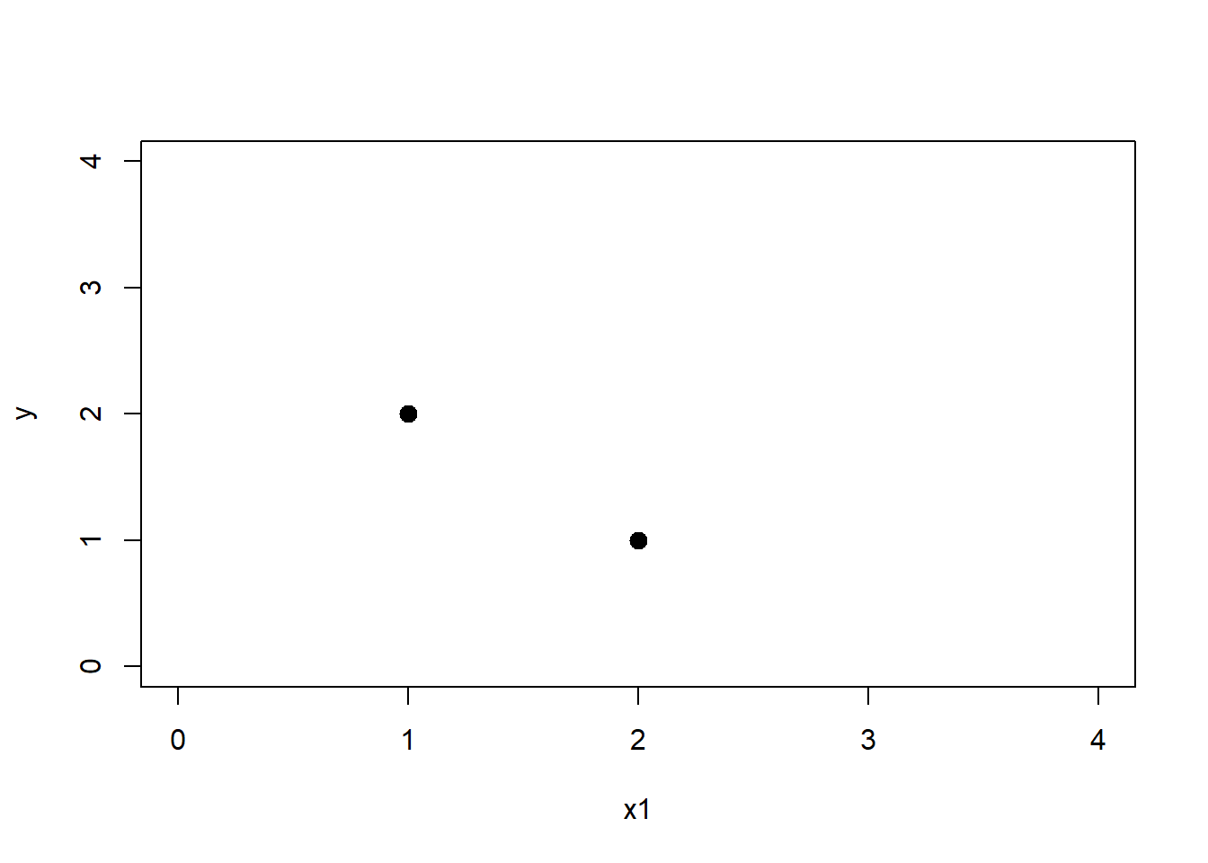
Here is clear that a regression line will connect the first point (in x1 = 1 and y = 2) and the second point (in x1 = 2 and y = 1). So in our line for every unit of \(x1\) (from x = 1 to x = 2) we descend 1 unit of \(y\) (from y = 2 to y = 1) and when x = 0 (the intercept) y should be equal to 3. Let’s make that plot, where the intercept = 3 and for each unit of x, y descends one unit (-1)
# Create data
x1 <- matrix(data = c(1,2))
y <- matrix(data = c(2,1))

# Plot points
plot(x1,y,pch = 20, xlim = c(0,4), ylim = c(0,4),cex = 2)
abline(a = 3,b = -1,col = 'red')
Perfect! But that seems too easy because we only have two points. A line can explain the relationship of two points perfectly by passing through both points. But what happens when there’s a third point that can’t go through all the points? If we used the previous line, that extra point would be separated from the regression line by a small distance. That distance is called residual.
# Create data
x1 <- matrix(data = c(1,2,1.5))
y <- matrix(data = c(2,1,1.75))

# Plot points
plot(x1,y,pch = 20, xlim = c(0,4), ylim = c(0,4),cex = 2)

# Draw Regression line
abline(a = 3,b = -1,col = 'red')

# Draw Residuals and text
segments(x0 = 1.5,x1 = 1.5,y0 = 1.75, y1 = 1.5,col = "blue",lwd = 3)
text(1.6,1.6,"Residual 'e_2'",pos = 4)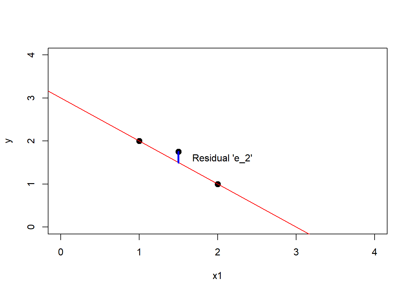
If we moved the slope of the regression, then the residuals of the other points would grow. If you see the blue line, that’s the perpendicular from each point to the regression line. Now consider that the value of the red line in the y-axis for every point in the x-axis (x1 variable) it’s our prediction, will refer to it as \(\hat y\) (y-hat). You can think of a regression as an input output machine. When I input a \(x=1\), my machine outputs a \(\hat y=2\). When I input a \(x=2\), my machine outputs a \(\hat y=1\), when I input a \(x=3\) then my machine produces a \(\hat y=0\) and so on.
Now the real values of the \(y\) variable are \(2,1.75\) and \(1\), and the values of \(\hat y\) are \(2,1.5\) and \(1\). So the residuals \(e_i\) are \(e_i = y_i - \hat y_i\) are \(2-2 = 0, 1.75 - 1.5 = .25, 1 - 1 = 0\), so \(0,0.25\) and \(0\). If we sum all the values (the sum of the residuals) the total would be \(0.25\)
Instead, we almost always will want to minimize the residual sum of squares \((y - \hat y)^2\). (By the way the sum of squares in our previous example would be \(0^2 + 0.25^2 + 0^2 = 0.0625\))
Question 1: Why do we want to minimize the residual sum of squares in regression?
Solution 1: When we do regression we want to minimize the sum \(e_i\). But if we only sum the residuals then the best regression would be the mean value of \(y\) (normally depicted as \(\bar y\)). That will not capture the relationship between x and y, because it’s a constant, or in the graph a horizontal line. That’s why instead we want to use the residual sum of squares.
Want to see an example? Look at the blue lines (the residuals of each point). If you sum their values, the negatives cancel the positive values, and as a result the best regression line is the mean value of \(y\)
# Create data
x1 <- matrix(data = c(1,2,1.5))
y <- matrix(data = c(2,1,1.75))
y_bar <- mean(y)
# Plot data
plot(x1,y,pch = 20, xlim = c(0,4), ylim = c(0,4),cex = 2)
# Regress with sum of residuals
abline(a = y_bar,b = 0,col = 'red')
# Draw residuals
segments(x0 = 1,x1 = 1,y0 = 2, y1 = y_bar,col = "blue",lwd = 3)
segments(x0 = 1.5,x1 = 1.5,y0 = 1.75, y1 = y_bar,col = "blue",lwd = 3)
segments(x0 = 2,x1 = 2,y0 = 1, y1 = y_bar,col = "blue",lwd = 3)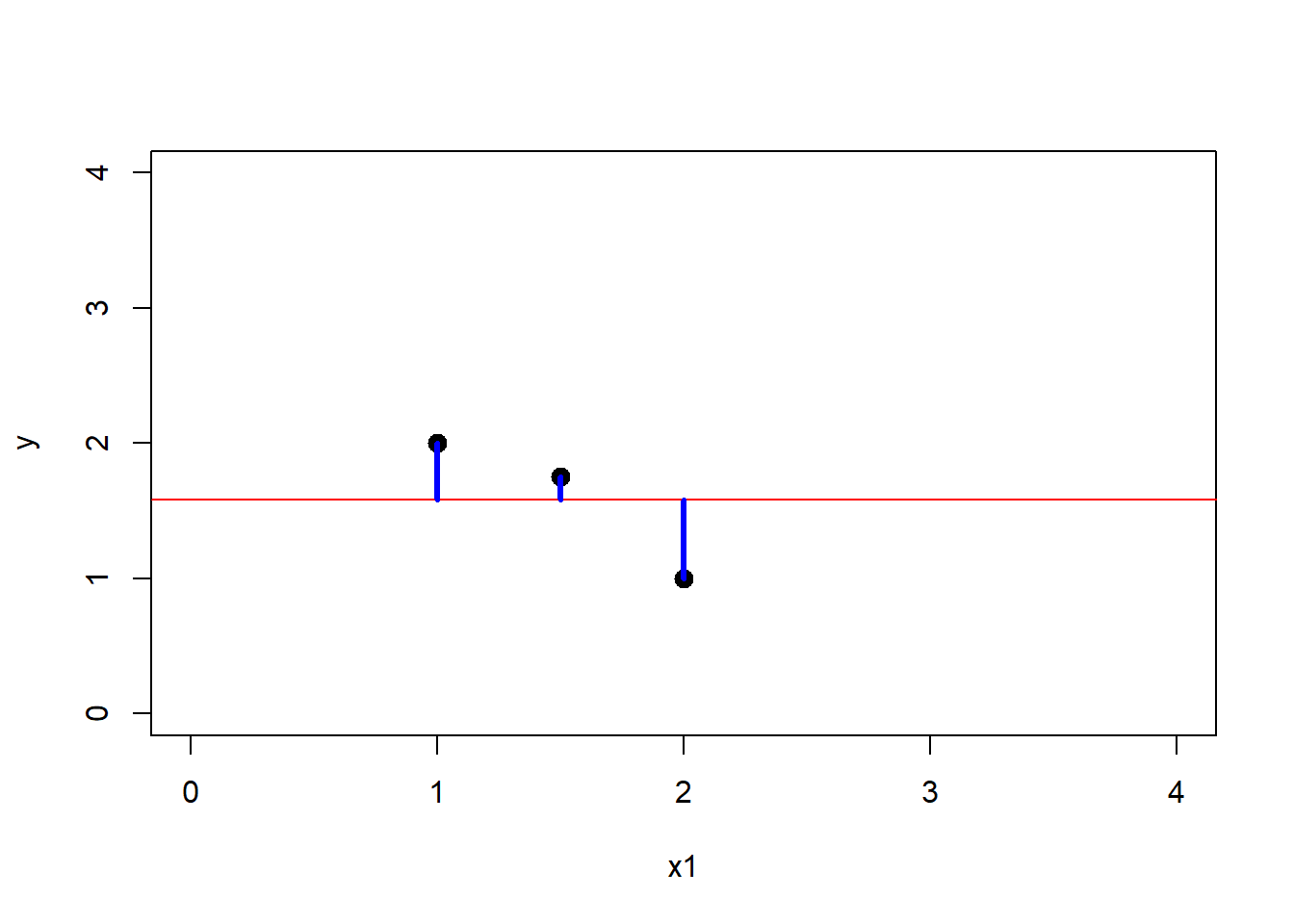 Let’s do the numerical exercise.
The mean value of \(y =\) 1.58 \(= \hat y\)
If we sum all these blue bars \(e_i\) (where i indicates the residual of each point \(e_1\) is the residual of the point (x=1,y=2), \(e_2\) the residual of (1.5,1.75) and \(e_3\) the residual of (2,1)), the result would be \(e_1 = 2 - 1.58\) , \(e_2 = 1.75 - 1.58\) , \(e_3 = 1.75 - 1.58\) If we sum the residuals then 0.42 + -0.58 + 0.17 = 0
Instead we can use two strategies, either sum the absolute values of the residuals \(\sum \mid y - \hat y \mid\) or the residual sum the squares \(\sum (y - \hat y)^2\) also denoted as \(\mid\mid\ y - \hat y \mid\mid^2\) which is the norm of the residuals, more on this later. In a different post we will explore the pros and cons of each one of them. But for now just remember that square of the residuals will penalize values that are far away, that way the line will cross the cloud of points. For now on, we will focus in this second one.
As we saw, sometimes the best regression line will not fit perfectly every point. That means that the \(y\) is not in the column space of \(x1\) variable. That means that there isn´t any linear combination of \(x1\) that predicts \(y\) perfectly. What do we do instead? We predict \(\hat y\) which is the closest projection of \(y\) to the column space of \(x1\) and \(x_0\).
I use here a value for \(x_0\) because you can interpret the intercept as a variable that always takes the value 1 like in this plot:
x0 <- matrix(data = c(1,1))
y <- matrix(data = c(2,1))
plot(x0,y,pch = 20, xlim = c(0,4), ylim = c(0,4),cex = 2)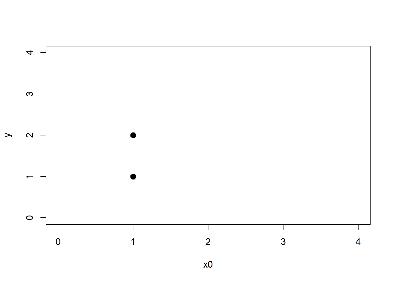
Question 2: How do we minimize the residual sum of squares in regression?
Solution 2 We have to project the \(y\) results on the column space of \(X\)
Let’s start more slowly.We basically we want to predict the following form:
\[\hat y = \beta_0x_0 + \sum_{i=1}^p{X_i \beta_i} \] Where \(\hat y\) is the closest or equal to \(y\). We want a value \(\hat y\) such that \((y - \hat y)^2\) is as small as possible.
This means that an intercept \(\beta_0\) + the product of all the dependent variables we have times their coefficient \(\beta_i\) will produce the projection \(\hat y\) closest to the actual y.
If we go back to our original example with two points. \(\beta_0\) it’s the the intercept = 3, and we only have 1 variable to predict so p = 1, because we only have one variable we only calculate 1 coefficient \(\beta_1\), which we saw it was -1. We can calculate then for example when our variable \(x1\) = 1 we see that our formula spits out \(\hat y = \beta_0 + {X_1 \beta_1} = 3 + 1 * -1 = 2\). So conveniently this choice of \(\beta_0 = 3\) and \(\beta_1 = -1\) help us predict a value \(\hat y\) that it’s the same as the actual \(y\). But in this case it was easy to do because there was a line that predicted every point. But how do we go about if there isn’t any combination of \(\beta_0\) and \(\beta_1\) that perfectly predicts \(y\)? In this case, mathematically speaking, it means \(y\) doesn’t lie in the column space of \(x_0\) and \(x_1\) and we need to find the value for each \(\beta\) that give us the \(\hat y\) closest to \(y\)
Question 2.1 What is the column space?
Solution The column space is every linear combination of predictor variables \(x_0\) and all the other \(x_i\). From now on when I refer to predictor variables I will show it as a big \(X\). Which can be represented as a matrix: \[\begin{pmatrix} 1 & 1 \\ 1 & 2 \end{pmatrix}\]
The first column is the values of \(x_0\) and the second the values of \(x_1\). If we had more columns we would add more values. Then the column space would be the resulting space that could be predicted if we chose every value of \(\beta\). Let’s check an example. Imagine we are in the original data set with two points. To visually understand column space let’s choose one value for \(\beta_0\) like 3 and let’s pick a few values of \(\beta_1\) to see the different lines
x0 <- matrix(data = c(1,1))
x1 <- matrix(data = c(1,2))
y <- matrix(data = c(2,1))
plot(x1,y,pch = 20, xlim = c(0,4), ylim = c(0,4),cex = 2)

vals <- seq(-10,10,length.out = 110)
#vals <- seq(-10^2,10^2,length.out = 220)
for( i in vals){
  abline(a = 3,b = i,col = 'red') # Line one
}
All the red lines and the space in between represent the column space of \(x_1\) (if the origin was fixed = 3). Meaning all the vectors we could create by choosing different values of \(\beta_1\). We see that there’s at least one line that passes through both points \(y_1,y_2\) that means that \(y\) which can be seen as a matrix like before \(\begin{bmatrix}2 \\ 1\end{bmatrix}\) it’s in the column space of \(X = \begin{pmatrix} 1 & 1 \\ 1 & 2 \end{pmatrix}\) because there’s a combination of betas \(\begin{bmatrix}\beta_0 \\ \beta_1\end{bmatrix} = \begin{bmatrix}3 \\ -1\end{bmatrix}\) that multiplied by \(X= \begin{pmatrix} 1 & 1 \\ 1 & 2 \end{pmatrix}\) will produce the same output \(\hat y = y = \begin{bmatrix}2 \\ 1\end{bmatrix}\). So we can draw this in matrix form like: \[X \beta = y\] where lower case indicates a matrix of one column (a vector) and upper case is a matrix of 2 or more columns. The numeric example would be \[\begin{pmatrix} 1 & 1 \\ 1 & 2 \end{pmatrix} \begin{pmatrix}\ 3 \\ -1\end{pmatrix} = \begin{pmatrix}2 \\ 1\end{pmatrix}\]
Remember that matrix multiplication is always rows times columns so its equivalent to \(1*3 + 2*-1 = 2\) and \(1*3 + 1*-1 = 1\) For more on Linear Algebra and Matrices I highly recommend the videos of @3blue1brown on matrix multiplication. He explains visually how this works
So for this case we were lucky that \(y\) was on the column space or plainly speaking in the plane \(X\beta\) but what happens when we have something like this
x0 <- matrix(data = c(1,1,1))
x1 <- matrix(data = c(1,2,1.5))
y <- matrix(data = c(2,1,1.75))
plot(x1,y,pch = 20, xlim = c(0,4), ylim = c(0,4),cex = 2)
vals <- seq(-10,10,length.out = 110)
#vals <- seq(-10^2,10^2,length.out = 220)
for( i in vals){
  abline(a = 3,b = i,col = 'red') # Line one
}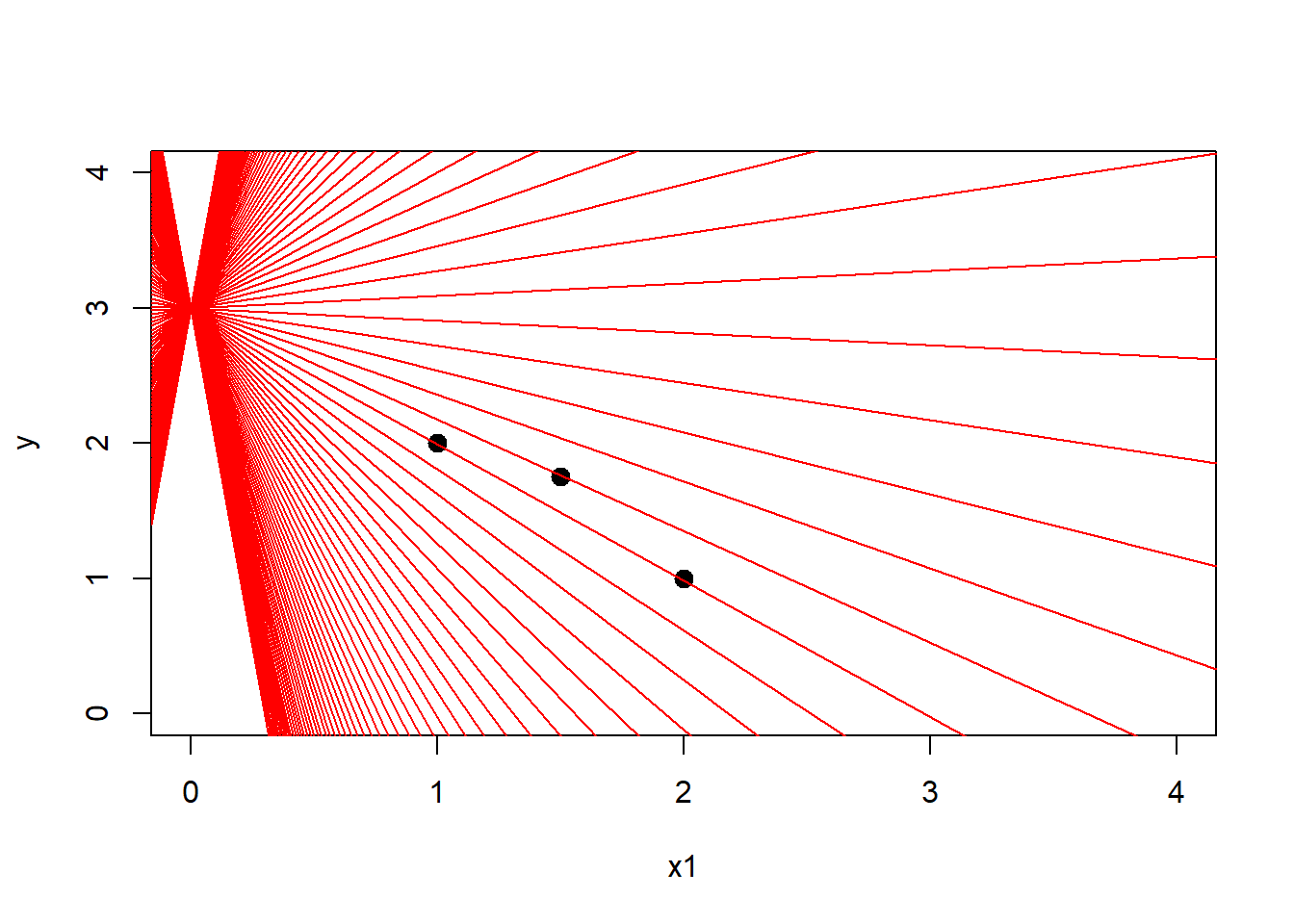
Here, even though we have several lines that pass close to all the points. There isn’t any line that passes through all the points at the same time. Which means there isn’t any combination of \(\beta\) that will result in the vector \(y\). If you imagine the column space of \(X\) as a flat sheet of possible vectors and \(y\) as a vector that does not lie in the same sheet it could be troublesome to imagine the translation from the 2D graph. The reason is you have to imagine one vector made of 3 points that is pointing upward in that sheet
This 3D visualization might be hard to understand but it will help you transition from the previous graph.
The red planes are the column space of \(X\) when we keep \(x0\) fixed
However, there isn’t a single red plane that can express the real solution (plane in blue), since this blue plane can’t be formed with a linear combination of \(x0\) and \(x1\)
Real Solution vs Column Space X
So which of the red planes we should pick? If the blue plane means no residuals, but this can’t be accomplished by the red planes. Our best model will be the red plane that is closest to the blue solution. But this is really hard to see from this view. Instead why don’t we twist the way we are looking at the data. Instead of looking at the columns as the coordinate system, we can see each axis as a vector, drawn in the coordinate system of the rows. This may give you a headache at first glance but let’s take it slowly.
Take each variable: \[x_0 = \begin{pmatrix} 1 \\ 1 \\ 1\end{pmatrix} x_1 = \begin{pmatrix} 1 \\ 1.5 \\ 2 \end{pmatrix} y = \begin{pmatrix} 2 \\ 1.75 \\ 1 \end{pmatrix}\]
Each row could be view as an axis of the coordinate system \(r_1\) \(r_2\) \(r_3\)
So if we represent each variable in this coordinate system as a vector we could see this.
Here the blue arrow is the target variable \(y\) and the other two red arrows are the variables \(x_0\) and \(x_1\), when we multiply any arrow by a number (a scalar) the result is a new arrow with a new span. When you combine both red arrows you will get a third arrow in the span of the red plane. But as you can see there, there’s no arrow that will land on the same place of the blue arrow. As before there’s no solution where residuals will be 0 (the blue arrow).
Let’s sketch this same view, to see this more clearly. We can see again how the \(y\) vector is not in the column space X.
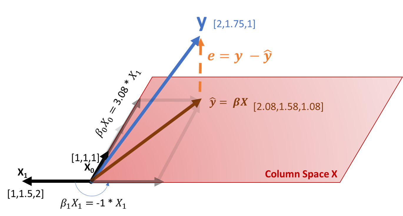
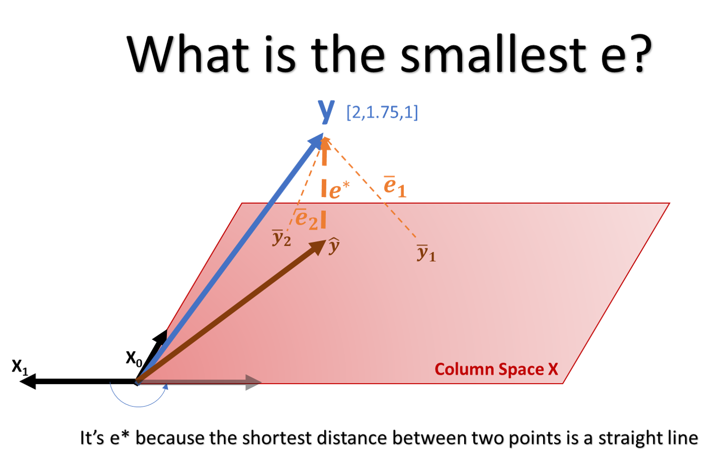
Then what is the best \(\hat y\) that minimizes the error? In other words, what vector in the red plane (the column space) would be best if we can achieve the blue vector? Well the shortest line you can draw from \(y\) to the column space of \(X\) it’s the perpendicular line from \(y\) to the column space. The same that the shortest distance between two points it’s a straight line, the shortest distance between a point and a plane is the perpendicular line from that point to the plane. Now instead of having a coefficient \(\beta\) to calculate \(y\) we will have coefficient \(\hat \beta\)(beta hat) to calculate \(\hat y\) like \(\hat y = X \hat \beta\). We call it \(\hat \beta\) because the outputted vector will be \(\hat y\) which is not exactly \(y\), but is the projection on the column space.
I bet you are probably thinking; Wait wait wait, in this tutorial we were going really slow through the explanation and all of a sudden I can’t connect the dots between this picture

and the geometrical interpretation we just saw?
Think about it this way, if there´s a plane that fits perfectly the 3 points in \(y\) but it´s impossible to create with the \(X\) variables, then the best regression line (that minimizes the magnitude of the residuals) in the \(X\) column space is the perpendicular projection of the vector \(y\) on the \(X\) column space plane. That is the essence of Least Squares. The line that minimizes the residual sum of squares is the orthogonal (aka perpendicular) projection of \(y\) on the column space \(X\)
Question 3: How do we calculate the orthogonal projection?
Solution 3: The orthogonal projection is equivalent to the inner product of the column space \(X\) and the error.
Let’s break this down slowly. If we project the vector of the residual \(e\) on to the plane the result will be 0. Because the vector of \(e\) spans perpendicular to the column space \(X\) plane. So the vector is 0. How do we do a perpendicular projection? In Euclidean spaces (our everyday spaces) with the dot product, that is equivalent to the inner product. In this case we want to project the residual e on the column space, with the dot product.
This is represented as \(\langle X,e\rangle= 0\) which is the equivalent of multiplying every item of \(X\) with the item of \(e\) and adding all together. Another way of doing this is by transposing the \(X\) Matrix (flipping it sideways) and doing matrix multiplication as before. Let’s do this
\[\langle X,e\rangle = X^Te = \begin{pmatrix} x_{01} & x_{11} \\ x_{02} & x_{12} \end{pmatrix}^T \cdot \begin{pmatrix}\ e_0 \\ e_1\end{pmatrix} = \begin{pmatrix} x_{01} & x_{02} \\ x_{11} & x_{12} \end{pmatrix} \cdot \begin{pmatrix}\ e_0 \\ e_1\end{pmatrix} = \begin{pmatrix} 1 & 1 \\ 1 & 2 \end{pmatrix} \cdot \begin{pmatrix}\ e_0 \\ e_1\end{pmatrix} = \begin{pmatrix}1*e_0 + 1*e_0 \\ 1*e_1 + 2*e_1\end{pmatrix}\] Take time to do this yourself and understand what is the Transpose doing and why is that equivalent to the dot product. To know more about the dot product see this video from @3blue1brown on dot product.
Next, we know that \(X^Te = 0\) and we know that \(e = y - \hat y\) moreover \(\hat y = X\hat\beta\) putting it all together we have that
\[X^T(y - X\hat\beta) = 0\] With a little algebra we can solve this equation like this
\[X^Ty - X^TX\hat\beta = 0\\ X^Ty = X^TX\hat\beta \\ \hat \beta = \frac{X^Ty}{X^TX} = (X^TX)^{-1} X^Ty \]
This \(\hat\beta = (X^TX)^{-1} X^Ty\) is the most important formula to learn. And because we are using matrix notation it’s valid for 1 variable or 100 variables.
So let’s go and calculate the \(\hat \beta\) using the previous formula.
# Create the data
x0 <- matrix(data = c(1,1,1))
x1 <- matrix(data = c(1,2,1.5))
y <- matrix(data = c(2,1,1.75))

X <- cbind(x0,x1)

# Calculate Beta hat
beta_hat = solve(t(X) %*% X) %*% t(X) %*% y  # the simbol %*% indicates matrix multiplication and solve() indicates inverse ^-1

#Label the rows and column
dimnames(beta_hat) <- list(c("beta_0 (Intercept)","beta_1"),"Coefficients")

# Print Result
beta_hat
## Coefficients
## beta_0 (Intercept) 3.083333
## beta_1 -1.000000Now we can predict our \(\hat y\) by multiplying \(X\) by \(\hat \beta\). Let’s see the result.
# Create the data
x0 <- matrix(data = c(1,1,1))
x1 <- matrix(data = c(1,2,1.5))
y <- matrix(data = c(2,1,1.75))

X <- cbind(x0,x1)

# Calculate Beta hat
beta_hat = solve(t(X) %*% X) %*% t(X) %*% y  # the simbol %*% indicates matrix multiplication and

# Calculate Y hat
y_hat = X %*% beta_hat

# Print
y_hat
## [,1]
## [1,] 2.083333
## [2,] 1.083333
## [3,] 1.583333How does this look like in our original plot. Let’s see the Least Squares solution in orange.
# Create data
x0 <- matrix(data = c(1,1,1))
x1 <- matrix(data = c(1,2,1.5))
y <- matrix(data = c(2,1,1.75))
X <- cbind(x0,x1)

# Calculate Beta hat
beta_hat = solve(t(X) %*% X) %*% t(X) %*% y  # the simbol %*% indicates matrix multiplication and

# Calculate Y hat
y_hat = X %*% beta_hat

# Plot points
plot(x1,y,pch = 20, xlim = c(0,4), ylim = c(0,4),cex = 2)

# Draw Original Regression line
abline(a = 3,b = -1,col = 'red')

# Draw new Least Squares Solution
abline(a = beta_hat[1],b = beta_hat[2],col = 'orange', lwd = 2)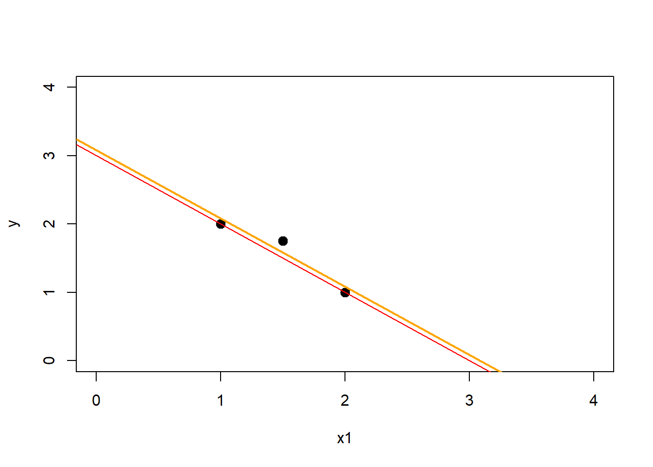
Here even though it doesn’t look like much we have a smaller residuals sum of squares. Should we calculate it?
# Create data
x0 <- matrix(data = c(1,1,1))
x1 <- matrix(data = c(1,2,1.5))
y <- matrix(data = c(2,1,1.75))
X <- cbind(x0,x1)

# Calculate Beta_hat and y_hat
beta_hat = solve(t(X) %*% X) %*% t(X) %*% y  # the simbol %*% indicates matrix multiplication and
y_hat = X %*% beta_hat

# Calculate suboptimal Y-hat with coefficients Intercept = 3 slope = -1
beta2 <- matrix(data = c(3,-1))
y_hat2 = X %*% beta2


# Calculate residuals for Least Squares
RSS_yhat = sum((y-y_hat)^2)
# Calculate residuals for subOptimal Solution
RSS_yhat2 = sum((y-y_hat2)^2)

# Print
print(paste("RSS of yhat:",RSS_yhat))
## [1] "RSS of yhat: 0.0416666666666667"print(paste("RSS of sub-optimal yhat:",RSS_yhat2))## [1] "RSS of sub-optimal yhat: 0.0625"How will this be represented in the 3D view we had before? In the original \(x_0\),\(x_1\),\(y\), the solution would look like this
Where the optimal solution is the blue plane, and the projected solution is the orange, which coincides with one of the potential solutions of the red planes depicted.
We can do one more trick. If \(\hat y = X \hat \beta\) then \(\hat y = X (X^TX)^{-1} X^Ty\). This piece \(X (X^TX)^{-1} X^T = H\) it’s called Hat Matrix because it puts the hat on the \(y\). \(\hat y = Hy\) and it’s going to tell us a lot of things about the projection \(\hat y\). The geometrical interpretation is that is the orthogonal projection onto the column space (see above for how we get to this conclusion). It’s going to tell us how different \(y\) and \(\hat y\) will be. The Hat Matrix will explain the variance used from each of the variables, and the covariance from each of the combination of the \(X\) variables, and one very important feature: We can find how to do a regression line with only one variable. I know it seems silly to have solved then N-dimensional solution try to now figure out the 1-dimensional solution. But going the other way around will miss the visual interpretation of Least Squares.
Question 4: How do you calculate the Simple linear Regression with one variable?
Solution 4: If \(X\) only has one column \(x1\) then the expression \(\hat \beta = (X^TX)^{-1} X^Ty\) can be thought of like this: * \(X^TX = x_1^Tx_1 = \langle x_1,x_1\rangle\) this is the same as Sum of Squares \(\sum x_1^2\) (remember the dot product is the same as multiplying each item by itself and adding the result) * \((X^TX)^{-1}\): if \(X^TX\) is the same as \(\sum x_1^2\) then \((X^TX)^{-1} =\frac{1}{X^TX} = \frac{1}{\sum x_1^2}\). And as we saw before if \(\sum x_1^2\) is the same as \(\langle x_1,x_1\rangle\) then \(\frac{1}{\sum x_1^2}\) is the same as \(\frac{1}{\langle x_1,x_1\rangle}\) * Finally the piece \(X^Ty\): could be thought of \(x_1^Ty\) or again \(\langle x_1,x_1\rangle\) which is again the dot product of \(x_1\) and \(y\) or \(\sum x_1y\)
Putting all together \(\hat \beta = \frac{\langle x_1,y\rangle}{\langle x_1,x_1\rangle}\) or \(\hat \beta = \frac{x_1^Ty}{x_1^Tx_1}\)
What’s more. If we use the form we learned that \(\hat y = H y\) where \(H = X(X^TX)^{-1} X^T\) this could be re-written as \(H = x_1 \frac{1}{\sum x_1^2} x_1^T\) (I’m mixing Matrix notation with simple notation which is wrong but I want you to get the point). Let’s see how this last operation will play out with numbers.
\[H = \begin{pmatrix}1\\1.5\\2 \end{pmatrix} \frac{1}{\sum x_1^2} \begin{pmatrix} 1 & 1.5 & 2 \end{pmatrix}\] If we do this by number then we will get the following. \(H_{11} = \frac{1 * 1}{1^2 + 1.5^2 + 2^2} = \frac{1}{7.25} = 0.138\) \(H_{12} = \frac{1 * 1.5}{1^2 + 1.5^2 + 2^2} = \frac{1.5}{7.25} = 0.207\) \(H_{13} = \frac{1 * 2}{1^2 + 1.5^2 + 2^2} = \frac{2}{7.25} = 0.275\) \(\cdots\) \(H_{33} = \frac{2 * 2}{1^2 + 1.5^2 + 2^2} = \frac{4}{7.25} = 0.552\)
The result is something like this: \[H = \begin{pmatrix}0.14 & 0.20 & 0.27 \\ 0.20 & 0.31 & 0.41 \\ 0.27 & 0.41 & 0.55 \end{pmatrix} \]
Do you see what this is? First notice that the diagonal values correspond to the point multiplied by itself (divided by the square of all the other points. This is equivalent of saying what proportion of the total \(\sum x_1^2\) does the each point represent. Could you guess what happens if the one of the points is abnormally big? What would be it’s value in the diagonal? The answer would be very big. But because each numerator is going to be a part of the total denominator, a value of this diagonal could only go as high as 0.999 or 1. Let’s try that out.
Imagine we change the last point from 2 to 20. What would happen to the equation?
\[H = \begin{pmatrix}1\\1.5\\20 \end{pmatrix} \frac{1}{\sum x_1^2} \begin{pmatrix} 1 & 1.5 & 20 \end{pmatrix}\]
\[H = \begin{pmatrix}0.00 & 0.00 & 0.05 \\ 0.00 & 0.01 & 0.07 \\ 0.05 & 0.07 & 0.99 \end{pmatrix} \] Now all of a sudden all the third point has a very high value in the diagonal, and the other values in the diagonal are almost 0. This is the leverage. The leverage is the degree of influence of the each point on each \(\hat y\) value prediction. This means that a diagonal value very high means that the slope will significantly change due to this point. You can find more information on the leverage and the degree of influence on the fitted value here
But what about the other points what do those mean? Well for example the value \(H_12\) is the influence of the point 1 on the fitted value 2. This is symmetrical to say the value \(H_21\) is the influence of the point 2 on the fitted value 1, because when the regression line pivots, one side goes up or down and the other side of the pivot goes in the opposite direction.
There’s a lot more about the Hat matrix \(H\) but we will talk about it in a future post.
Question 5: But I have seen that for the Simple linear Regression the slope \(\beta_1\) is equal to the covariance of x and y divided by variance of x written as \(\beta_1 = \frac{cov(x,y)}{var(x)}\) and that the intercept is the mean of \(y\) minus the \(\beta_1\) times the mean of x \(\beta_0 = \bar y - \beta_1 \bar x\) How is this related to the equations we saw before?
Solution 5: The intercept is the same thing as shifting the entire coordinate system up or down. So from the solution we had before
Because we have two variables the simplification we did on Question 4 gets a little more complicated. But let’s do this again. \(\hat \beta = (X^TX)^{-1} X^Ty\). Now I will refer to \(x_0\) as 1’s in a matrix, because it will make the calculations easier. I will do the formulas and below the code in R.
\(X= \begin{pmatrix} 1 & x_{11} \\ 1 & x_{12} \\ 1 & x_{13} \end{pmatrix}\)
\(X^TX = \begin{pmatrix} 1 & 1 & 1\\ x_{11} & x_{12} & x_{13} \end{pmatrix}\begin{pmatrix} 1 & x_{11} \\ 1 & x_{12} \\ 1 & x_{13} \end{pmatrix} = \begin{pmatrix} n & \sum x_1 \\ \sum x_1 & \sum x_1^2 \\ \end{pmatrix}\)
Let’s do this with numbers
# Create data
x0 <- matrix(data = c(1,1,1))
x1 <- matrix(data = c(1,2,1.5))
X <- cbind(x0,x1)

# Print X
print(X)
## [,1] [,2]
## [1,] 1 1.0
## [2,] 1 2.0
## [3,] 1 1.5#Print X^T X
t(X) %*% X## [,1] [,2]
## [1,] 3.0 4.50
## [2,] 4.5 7.25- \((X^TX)^{-1} = \frac{1}{n\sum x_1^2-(\sum x_1)^2} \begin{pmatrix} \sum x_1^2 & \sum x_1 \\ \sum x_1 & n \\ \end{pmatrix}\)
# Create data
x0 <- matrix(data = c(1,1,1))
x1 <- matrix(data = c(1,2,1.5))
X <- cbind(x0,x1)
Xb <- cbind(x1,-x0)

#Print (X^T X)^-1 form
way1 = solve(t(X) %*% X)
print(way1)
## [,1] [,2]
## [1,] 4.833333 -3
## [2,] -3.000000 2# Print in fraction form
frac = 1/(length(x0)*sum(x1^2)-(sum(x1)^2))
mat = t(Xb) %*% Xb
way2 = frac * mat
#identical?
if(sum(round(way1-way2,3))==0){paste("Identical")}else{"not Identical"}## [1] "Identical"- Finally \(X^Ty = \begin{pmatrix} 1 & 1 & 1\\ x_{11} & x_{12} & x_{13} \end{pmatrix}\begin{pmatrix} y_{1} \\ y_{2} \\ y_{3} \end{pmatrix} = \begin{pmatrix} \sum y \\ \sum yx_1 \end{pmatrix}\)
# Create data
x0 <- matrix(data = c(1,1,1))
x1 <- matrix(data = c(1,2,1.5))
X <- cbind(x0,x1)
Xb <- cbind(x1,-x0)

#Print (X^T X)^-1 form
xty = t(X) %*% y
print(xty)
## [,1]
## [1,] 4.750
## [2,] 6.625# Its the same as
xty_2 = matrix(c(sum(y),sum(x1*y)))
#Identical?
identical(xty,xty_2)## [1] TRUEIf we put all this together
\[\hat \beta = \frac{1}{n\sum x_1^2-(\sum x_1)^2} \begin{pmatrix} \sum x_1^2 & \sum x_1 \\ \sum x_1 & n \\ \end{pmatrix} \begin{pmatrix} \sum y \\ \sum yx_1 \end{pmatrix} \]
if we do some algebra we end up with
\[\hat \beta = \begin{pmatrix} \bar y - \frac{\sum(x_1-\bar x_1)(y - \bar y)}{\sum(x_1 - \bar x)^2}\bar x \\ \frac{\sum(x_1-\bar x_1)(y - \bar y)}{\sum(x_1 - \bar x)^2} \end{pmatrix} = \begin{pmatrix} \bar y - \frac{SP_{x_1y}}{SS_{x_1}}\bar x_1 \\ \frac{SP_{x_1y}}{SS_{x_1}} \end{pmatrix} = \begin{pmatrix} \hat \beta_0 \\ \hat \beta_1 \end{pmatrix} \]
You can see how the coefficient of \(\hat \beta_1\) is the covariance of \(x_1\) and \(y\) divided by the variance of \(x_1\) and the coefficient of the intercept is written in terms of \(\hat \beta_1\)
This is interesting because we can apply the same process to estimate what is the \(\hat H\) Hat matrix made of, and understand how is each of the individual \(h_{ij}\) influencing the final \(\hat y\)
That’s all. We went from the very basic to the more complicated definition of the formulation. There’s one more task we did not spend a lot of time explaining. How is the square of the residuals related to the Hat matrix. But you can find this yourself already. How? Well because if the \[RSS = \sum e^2 = e^Te = \langle e,e\rangle\]
and \[e = y - \hat y = y - X\hat\beta = y - X(X^TX)^{-1} X^Ty\]
then the square of \(e\) it’s equal to
\[ RSS = y^Ty - y^TX(X^TX)^{-1} X^Ty = y^T(I - H)y \]
# Create data
x0 <- matrix(data = c(1,1,1))
x1 <- matrix(data = c(1,2,1.5))
X <- cbind(x0,x1)

# Beta hat
beta_hat = solve(t(X) %*% X) %*% t(X) %*% y
y_hat = X%*%beta_hat

# hat Matrix
hat_matrix = X %*% solve(t(X) %*% X) %*% t(X)

# RSS via hat matrix
RSS_hat = t(y) %*% (diag(3) - hat_matrix) %*% y


# Hat matrix via sum of squares
RSS_yhat = sum((y-y_hat)^2)

#identical?
if(sum(round(RSS_hat-RSS_yhat,3))==0){paste("Identical")}else{"not Identical"}
## [1] "Identical"Short Solution:
Now that we have worked out how does it work. Let’s show the algebraic solution to Least Squares.
Imagine we have the output variable \(y = \begin{pmatrix} 2 \\ 1 \end{pmatrix}\) and the input variables \(X = \begin{pmatrix} 1 & 1 \\ 1 & 2 \end{pmatrix}\) where the first column represents the intercept and the second column is the second variable.
In order to do a least squares we need to find the values of \(\beta\) that minimize the residual sum of squares \(RSS(\beta) = \sum_{i=1}^{N} (y_i - \beta_0 - \sum_{j=i}^p x_{ij}\beta_j)^2\) or in matrix notation \(RSS(\beta) = (y - X\beta)^T(y-X\beta)\)
Differentiating with respect to \(\beta\) we obtain \[\frac{\partial RSS}{\partial\beta} = -2X^T (y - X\beta) \] If \(X\) is full rank then we can set the first derivative to zero \(-2X^T (y - X\hat \beta) = 0\). This zero doesn’t mean that the RSS will be zero, instead it means that the value we find its a minimum for the function. If we isolate \(\hat\beta\) we get that \[\hat \beta = (X^TX)^{-1}X^Ty \]
So let’s apply this to our data then
# Create Data
x0 <- matrix(data = c(1,1))
x1 <- matrix(data = c(1,2))
y <- matrix(data = c(2,1))
X <- cbind(x0,x1)

# Regress y on X
betas_X <- solve(t(X) %*% X) %*% t(X) %*% y

## If we compare this to the lm function in R
lm1 <- lm(y ~ X - 1) # Regression using lm function

## If we compare the results
t(betas_X)  # Result manual
## [,1] [,2]
## [1,] 3 -1coef(lm1) # Result lm function## X1 X2
## 3 -1Now can we predict \(\hat y\) with \(X\hat\beta\). And check how well we did compared to the original ?
# Multiply the variables by the coefficients
y_hat <- X %*% betas_X

#Let's see the results from the original
y
## [,1]
## [1,] 2
## [2,] 1# And the results from our prediction
y_hat## [,1]
## [1,] 2
## [2,] 1Pretty good! I mean it’s a simple example but if we get exactly what’s going on we will be able to give a better interpretation to the outputs we get when we do regression in any statistical software.
